Appendix A — The Bootstrap

Work-in-progress 🚧

You are reading the work-in-progress first edition of Causal Inference in R. This chapter has its foundations written but is still undergoing changes.

A.1 Overview

The bootstrap is a simple but flexible algorithm for calculating statistics using resampling with replacement. It’s handy when a closed-form solution doesn’t exist to calculate something, as is commonly the case in causal inference (particularly for standard errors), or when we suspect the assumptions used for a parametric approach are not valid for a given situation.

Bootstrapping in R has a long tradition of writing functions to calculate the statistic of interest, starting with the classic boot package. Throughout the book, we’ll use rsample, a more modern alternative for resampling, but generally, we start with writing a function to calculate the estimate we’re interested in.

Let’s say we want to calculate some_statistic() for this_data. To bootstrap for R resamples, we:

1. Resamplethis_data with replacement. The same row may appear multiple (or no) times in a given bootstrap resample, simulating the sampling process in the underlying population.

   indices <- sample(
     # create a vector of indices:
     # 1 through the number of rows
     seq_len(nrow(this_data)), 
     # sample a vector indices 
     # that's the same length as `this_data`
     size = nrow(this_data), 
     replace = TRUE
   )
   bootstrap_resample <- this_data[indices, ]

2. Fit some_statistic() on the bootstrap_resample

   estimate <- some_statistic(bootstrap_resample)

3. Repeat R times

We then end up with a distribution of estimates, with which we can calculate population statistics, such as point estimates, standard errors, and confidence intervals.

A.2 Bootstrapping with rsample

rsample is a resampling package from the tidymodels framework, but it works well for problems outside of tidymodels. It has a little more overhead than the boot package, but consequently, it’s more flexible.

Let’s say we have some sampled data with three variables, x, z, and y, and we want to calculate confidence intervals for the coefficients of x and z in a linear regression with the outcome as y. We can calculate them using the bootstrap (in addition to the closed-form solutions provided with R).

library(tidyverse)
library(rsample)
set.seed(1)
n <- 1000
sampled_data <- tibble(
  z = rnorm(n),
  x = z + rnorm(n),
  y = x + z + rnorm(n)
)

lm(y ~ x + z, data = sampled_data)

Call:
lm(formula = y ~ x + z, data = sampled_data)

Coefficients:
(Intercept)            x            z  
     0.0162       1.0220       1.0270  

First, we use the bootstraps() function to create a nested dataset with each resampled dataset stored as rsplit objects.

bootstrapped_resamples <- bootstraps(sampled_data, times = 10)

bootstrapped_resamples$splits[[1]]

<Analysis/Assess/Total>
<1000/373/1000>

Here, the first bootstrapped dataset contains 627 of the original rows, and 373 were not included. If we look at the resulting data frame, we see 1000 rows, the same as in the original dataset. That means that some of the included rows are there more than once; each row is sampled with replacement. This spread is close to what we expect on average: about two-thirds of the original dataset ends up in each bootstrapped dataset.

boot_resample <- bootstrapped_resamples$splits[[1]] |>
  as.data.frame()

boot_resample

# A tibble: 1,000 × 3
         z      x      y
     <dbl>  <dbl>  <dbl>
 1  0.244   0.742  0.194
 2  0.984   0.971  2.84 
 3 -1.59   -2.33  -3.66 
 4 -0.0109 -1.47  -0.885
 5  0.391   0.373  2.99 
 6 -0.737  -2.64  -3.34 
 7  0.992   1.53   1.92 
 8  0.525  -1.12  -3.17 
 9  0.0773  0.927 -0.801
10 -1.28   -1.84  -4.69 
# ℹ 990 more rows

As described in the algorithm in Section A.1, we’ll fit the model on each bootstrapped dataset.

lm(y ~ x + z, data = boot_resample)

Call:
lm(formula = y ~ x + z, data = boot_resample)

Coefficients:
(Intercept)            x            z  
     0.0245       0.9812       1.0559  

Let’s express this as a function.

fit_lm <- function(.split) {
  .df <- as.data.frame(.split)
  lm(y ~ x + z, data = .df)
}

bootstrapped_resamples$splits[[1]] |>
  fit_lm()

Call:
lm(formula = y ~ x + z, data = .df)

Coefficients:
(Intercept)            x            z  
     0.0245       0.9812       1.0559  

Rather than doing this one by one, we’ll use iteration to run the regression on each resample. bootstrapped_resamples$splits is a list, so we could iterate over that with map() and get a list back. bootstrapped_resamples$splits is specifically a list-column, a list that is a column in a data frame. We’ll take advantage of the existing structure in bootstrapped_resamples to store the results as another list-column.

bootstrapped_resamples <- bootstrapped_resamples |>
  mutate(lm_results = map(splits, fit_lm))

Now each element of lm_results is an lm object—the regression fit to the bootstrapped resample. Here’s the model from the last resample.

bootstrapped_resamples$lm_results[[10]]

Call:
lm(formula = y ~ x + z, data = .df)

Coefficients:
(Intercept)            x            z  
     0.0341       1.0381       1.0005  

Now, we have ten estimates of each of the three coefficients in the model (the intercept, x, and z). Figure A.1 presents their distributions.

library(broom)
bootstrapped_resamples <- bootstrapped_resamples |>
  mutate(tidy_results = map(lm_results, tidy))

unnested_results <- bootstrapped_resamples |>
  select(id, tidy_results) |>
  unnest(tidy_results)

unnested_results

# A tibble: 30 × 6
   id      term  estimate std.error statistic   p.value
   <chr>   <chr>    <dbl>     <dbl>     <dbl>     <dbl>
 1 Bootst… (Int…  0.0245     0.0321    0.762  4.46e-  1
 2 Bootst… x      0.981      0.0313   31.4    6.66e-151
 3 Bootst… z      1.06       0.0443   23.8    1.15e- 99
 4 Bootst… (Int…  0.0275     0.0329    0.834  4.04e-  1
 5 Bootst… x      1.04       0.0311   33.3    4.86e-164
 6 Bootst… z      0.997      0.0448   22.3    2.03e- 89
 7 Bootst… (Int…  0.00339    0.0340    0.0997 9.21e-  1
 8 Bootst… x      1.08       0.0318   33.9    5.10e-168
 9 Bootst… z      0.968      0.0466   20.8    5.88e- 80
10 Bootst… (Int…  0.00546    0.0321    0.170  8.65e-  1
# ℹ 20 more rows

unnested_results |>
  ggplot(aes(estimate)) +
  geom_density(fill = "steelblue", color = NA) +
  facet_wrap(~term, scales = "free")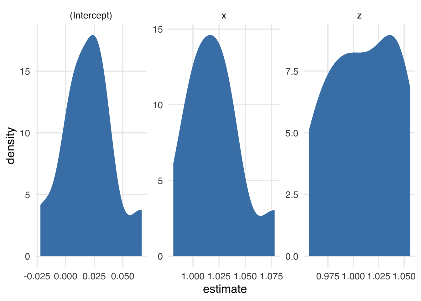

Figure A.1: The bootstrapped distributions of the coefficients from the model lm(y ~ x + z, data = .df). The distributions were calculated with 10 bootstrapped resamples.

The more times we resample, the smoother the distribution of estimates. Here’s 1000 times (Figure A.2).

bootstrapped_resamples_1k <- bootstraps(
  sampled_data,
  times = 1000
) |>
  mutate(
    lm_results = map(splits, fit_lm),
    tidy_results = map(lm_results, tidy)
  )

bootstrapped_resamples_1k |>
  select(id, tidy_results) |>
  unnest(tidy_results) |>
  ggplot(aes(estimate)) +
  geom_density(fill = "steelblue", color = NA) +
  facet_wrap(~term, scales = "free")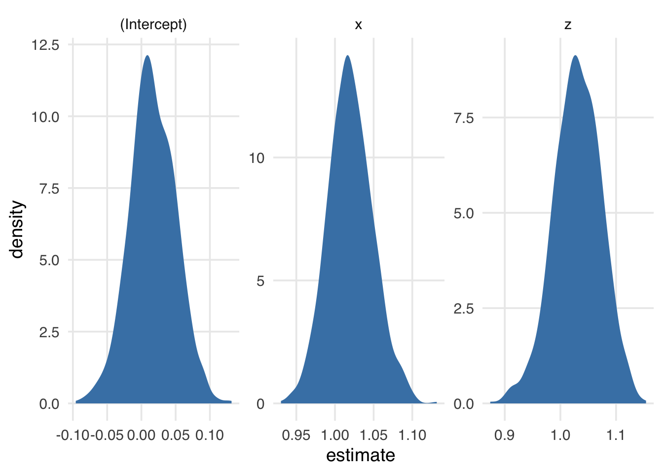

Figure A.2: The bootstrapped distributions of the coefficients from the model lm(y ~ x + z, data = .df). The distributions were calculated with 1000 bootstrapped resamples.

We can calculate information about the spread of these coefficients using the confidence interval functions in rsample, which follow the pattern int_*(nested_results, list_column_name). rsample expects the result to be either the results of broom::tidy() or a data frame with similar columns.

Let’s get simple percentile-based confidence intervals with int_pctl(). These will get the lower 2.5% and upper 97.5% quantiles.

int_pctl(bootstrapped_resamples_1k, tidy_results)

# A tibble: 3 × 6
  term         .lower .estimate .upper .alpha .method  
  <chr>         <dbl>     <dbl>  <dbl>  <dbl> <chr>    
1 (Intercept) -0.0511    0.0164 0.0824   0.05 percenti…
2 x            0.965     1.02   1.08     0.05 percenti…
3 z            0.941     1.03   1.11     0.05 percenti…

Now, we’ve got a data frame with each of our estimates and their bootstrapped confidence intervals. The remarkable thing about the bootstrap is that we can apply this recipe to an astonishing array of statistical problems, including problems that would otherwise be impossible to solve.

A.3 Why does it work?

Why does this remarkably simple algorithm work so well for so many problems? We direct you to the original paper and book on the bootstrap (Efron 1979; Efron and Tibshirani 1993) for the technical details. But let’s build some intuition for what’s happening.

Consider a population we want to understand. Sometimes, we have data on every observation in the population, but often, we need to sample the population, either out of necessity or efficiency.

library(tidyverse)
n <- 1000000
population <- tibble(
  z = rnorm(n),
  x = z + rnorm(n),
  y = x + z + rnorm(n)
)

population has a million observations, but we will randomly sample 200 observations from the whole population. If we need to conduct more sampling, we do so independently of the original sample. A given observation may end up in more than one study. Suppose 20 such studies have been done, all from the same population.

samples <- map(1:20, ~ population[sample(n, size = 200), ]) |>
  bind_rows(.id = "sample") |>
  mutate(sample = as.numeric(sample))

Because of random sampling variation, each sample’s mean of x is slightly different than in population, which is -6.8199^{-4}. Each of these sample estimates hovers around the population estimate (Figure A.3).

sample_means <- samples |>
  group_by(sample) |>
  summarize(across(everything(), mean))

samples |>
  ggplot(aes(x = x)) +
  geom_histogram() +
  geom_vline(
    data = sample_means,
    aes(xintercept = x),
    color = "firebrick"
  ) +
  facet_wrap(~sample)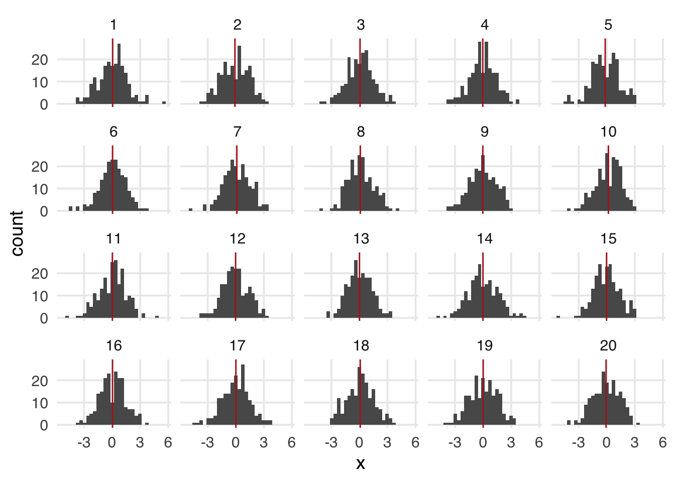

Figure A.3: The distributions of the sample means of x for twenty samples. Each sample is sampled from population and has a sample size of 200.

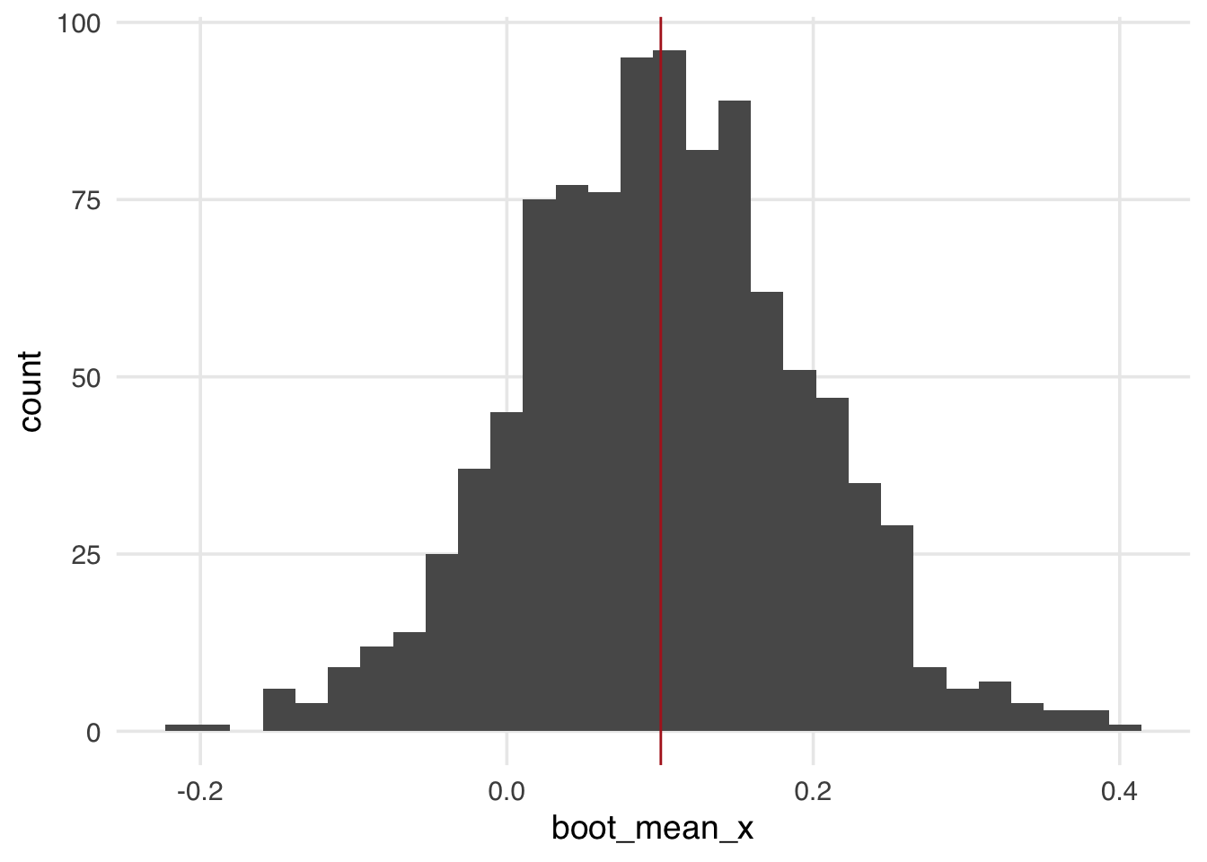
You may notice that sampling from the population bears a similarity to the sampling we do in the bootstrap. We’re treating the resample as representative of the population from which it comes. This helps us translate the distribution we see into terms of the original population, much the same way we get when we use parametric confidence intervals. A key difference from sampling the population is that the bootstrap will determine the spread around the sample estimate, not the population estimate. Let’s look at sample 8 a bit closer.

sample_8 <- samples |>
  filter(sample == "8")

sample_8 |>
  summarize(across(everything(), mean))

# A tibble: 1 × 4
  sample       z     x      y
   <dbl>   <dbl> <dbl>  <dbl>
1      8 -0.0406 0.100 0.0476

The sample mean of x is 0.1. Now, let’s bootstrap this sample and calculate the mean of x for each bootstrapped resample. The distribution of bootstrapped estimates in Figure A.4 falls symmetrically around the sample mean.

calculate_mean <- function(.split, what = "x", ...) {
  .df <- as.data.frame(.split)
  t <- t.test(.df[[what]])

  tibble(
    term = paste("mean of", what),
    estimate = as.numeric(t$estimate),
    std.error = t$stderr
  )
}

s8_boots <- bootstraps(sample_8, times = 1000, apparent = TRUE)
s8_boots <- s8_boots |>
  mutate(boot_mean_x = map(splits, calculate_mean))

s8_boots |>
  mutate(boot_mean_x = map_dbl(boot_mean_x, \(.df) .df$estimate)) |>
  ggplot(aes(x = boot_mean_x)) +
  geom_histogram() +
  geom_vline(
    data = sample_means |> filter(sample == "8"),
    aes(xintercept = x),
    color = "firebrick"
  )

Figure A.4: The bootstrapped distribution of x for a single sample. While we are simulating the sampling process from the underlying population, the distribution is centered around the sample mean, not the population mean.

Even though the distribution of estimates is around the sample mean, the bootstrap, by simulating the process of sampling from the population, grants us a population interpretation of the confidence intervals. A confidence interval is a frequentist concept related to multiple samplings from the same population. For 95% confidence intervals, 95% of confidence intervals estimated from samples will contain the actual population estimate. When this is true (e.g., 95 of 100 studies sampled from the population estimate confidence intervals that contain the population estimate), we say that the confidence intervals have nominal coverage.

For instance, let’s get the proportion of confidence intervals that contain the population mean of x. We’ll also increase the number of resamples to approximate the coverage better. (The more we increase the number of samples, the closer we’ll get to 95%.)

n_samples <- 1000

samples <- map(seq_len(n_samples), ~ population[sample(n, size = 200), ]) |>
  bind_rows(.id = "sample") |>
  mutate(sample = as.numeric(sample))

cis <- samples |>
  group_by(sample) |>
  group_modify(~ t.test(.x$x) |> tidy())

between(
  rep(mean(population$x), n_samples),
  cis$conf.low,
  cis$conf.high
) |>
  mean()

[1] 0.959

Bootstrapping allows us to attain confidence intervals with nominal coverage under many circumstances, the same as we see with the well-defined parametric approach above. We won’t run this since it requires r_bootstraps * n_samples calculations, but the results are similar.

bootstrap_ci <- function(.sample_df, ...) {
  sample_boots <- bootstraps(.sample_df, times = 1000)
  sample_boots <- sample_boots |>
    mutate(boot_mean_x = future_map(splits, calculate_mean))

  sample_boots |>
    int_pctl(boot_mean_x)
}

boot_cis <- samples |>
  group_by(sample) |>
  group_modify(bootstrap_ci)

coverage <- between(
  rep(mean(population$x), n_samples),
  boot_cis$.lower,
  boot_cis$.upper
) |>
  mean()

A.4 Why resampling with replacement?

People first encountering the bootstrap are often surprised to learn that we are resampling with replacement and that the same observation may appear in a bootstrapped sample more than once. The mathematic details are in the sources we cite above, but there are a few practical reasons to help build your intuition about why resampling with replacement works. Firstly, if you sampled without replacement, you would end up with the same estimate every time because you’d just have the original dataset. Jittering the samples varies the estimate. You could also sub-sample: sample a dataset without replacement smaller than the original dataset. However, this doesn’t work as well as resampling with replacement, although it can be useful for other problems. The reason why relates to the original population and how it’s sampled. Each sample is independent of one another, meaning an individual could end up in more than one sample. If you restricted the sample to individuals who were not in previous samples, your sampling scheme would no longer be independent; each sample would depend on the previous ones. Allowing each observation to be independent in resampling also lets it represent others like it in the original population, much like when we up-weight samples in inverse probability weighting (see Chapter 8.4).

A.5 How many bootstrapped resamples?

In this book, we use a thousand bootstrapped resamples for most problems to balance stability and computational speed. How many should you use in your real analysis?

You’ll often see older recommendations in the tens or hundreds of resamples, but these are from a time when processing power was more limited. On modern computers (even personal laptops), it’s practical to do many more. Hesterberg (2015) suggests a thousand resamples for rough estimates and ten to fifteen thousand resamples for when accuracy matters. By “accuracy,” we mean minimal variance due to the bootstrap simulation itself. A practical test for this is to try out R resamples more than once and increase R until you are satisfied with the degree of stability in your results.

Each bootstrap calculation is independent of the other, meaning that for a large number of resamples, you might want to use parallel processing. With the rsample approach we’ve shown, you can use furrr as a parallelized drop-in replacement for map(). furrr is a purrr-like API to the future framework.

library(future)
library(furrr)
n_cores <- availableCores() - 1
plan(multisession, workers = n_cores)

s8_boots <- s8_boots |>
  mutate(boot_mean_x = future_map(splits, calculate_mean))

A.6 Which confidence intervals to use?

Thus far, we’ve been using percentile-based confidence intervals. These are literally the 2.5% and 97.5% percentiles of the distribution of bootstrapped estimates. It’s fast, simple, and intuitive. However, several other types of bootstrap confidence intervals exist, and they can have better nominal coverage under some circumstances. rsample includes two others at the time of this writing: int_t() and int_bca(). int_t() calculates confidence intervals from the bootstrapped T-statistic. int_bca() calculates bias-corrected and accelerated confidence intervals.

You need estimates from the original data set for these types of confidence intervals. You can tell rsample to include the original one with bootstraps(data, times = 1000, apparent = TRUE) (we’ve already done that for s8_boots). That will result in 1001 datasets: the original plus 1000 bootstrapped datasets. For int_bca(), you also need to provide the function (to the .fn argument) you used to calculate the estimate, in this case, calculate_mean.

ints <- bind_rows(
  int_pctl(s8_boots, boot_mean_x),
  int_t(s8_boots, boot_mean_x),
  int_bca(s8_boots, boot_mean_x, .fn = calculate_mean)
)

ints

# A tibble: 3 × 6
  term       .lower .estimate .upper .alpha .method   
  <chr>       <dbl>     <dbl>  <dbl>  <dbl> <chr>     
1 mean of x -0.0875     0.102  0.286   0.05 percentile
2 mean of x -0.0829     0.102  0.295   0.05 student-t 
3 mean of x -0.0876     0.102  0.286   0.05 BCa       

In this case, the confidence intervals are very close. That’s because they all perform well for the normally distributed data like x.

A subtle detail of nominal coverage in confidence intervals is that the proportion of estimates that fall outside of the intervals should be roughly the same on either side of the confidence intervals. We see that, for instance, with confidence intervals from the traditional t-test for x.

c(
  mean(mean(population$x) < cis$conf.low),
  mean(mean(population$x) > cis$conf.high)
)

[1] 0.020 0.021

This symmetry doesn’t hold for many types of confidence intervals when the data are skewed. For example, a right-skewed distribution may result in nominal coverage of 95% for intervals but with 1% of the values below the lower bound (the left side of the distribution) and 4% above the upper bound (the right side of the distribution).

BCa intervals and bootstrap t-statistic intervals work better on skewed data. Notably, means approach the normal distribution as the sample size increases due to the central limit theorem regardless of the data’s distribution (although for skewed distributions, the required sample size can be in the thousands rather than the commonly cited 30). The same is often true of coefficients in regression models, which are conditional means. If the central limit theorem has taken effect, percentiles and other types of confidence intervals will likely also have good coverage.

When you have a result where you have reason to believe the bootstrapped distribution should look a certain way, such as means being normally distributed, it offers a potential diagnosis for your analysis. For instance, in causal inference, if you see a coefficient that is skewed or has another unexpected distribution, that may be a sign that you have a violation of the positivity assumption (see Chapter 3). Keep an eye out for unexpected instability between bootstrapped resamples.

Percentile and BCa intervals are transformation invariant, meaning that you can transform the estimate you bootstrapped and get the same result as if you had bootstrapped the transformation. An example of this is the log odds ratio versus the odds ratio. With a bootstrapped t-statistic interval, you may end up with different results depending on which you actually bootstrapped. So, if you’re working with data you want to view on more than one scale, you might want to use one of these.

A final consideration is computational speed. Percentiles are extremely fast and don’t require additional information. Bootstrap t-intervals and BCa intervals require information from the original dataset. The BCa is the most computationally intensive of the three. For many problems, the difference in speed is negligible on modern computers, but it may be useful to use percentile confidence intervals when you think they’d work well and BCa is taking a particularly long time.

A.7 When does the bootstrap not work out of the box?

The algorithm we’ve presented here is simple and powerful for many calculations, but some types of estimates are known not to work with the bootstrap or require a variation of the algorithm to calculate nominal confidence intervals. A typical example of this is extrema, such as the minimum or maximum value. For example, bootstrapping the minimum of x results in a strange distribution.

calculate_min <- function(.split, what = "x", ...) {
  .df <- as.data.frame(.split)

  tibble(
    term = paste("min of", what),
    estimate = min(.df[[what]])
  )
}

s8_boots <- s8_boots |>
  mutate(boot_min_x = map(splits, calculate_min))

s8_boots |>
  mutate(boot_min_x = map_dbl(boot_min_x, \(.df) .df$estimate)) |>
  ggplot(aes(x = boot_min_x)) +
  geom_histogram()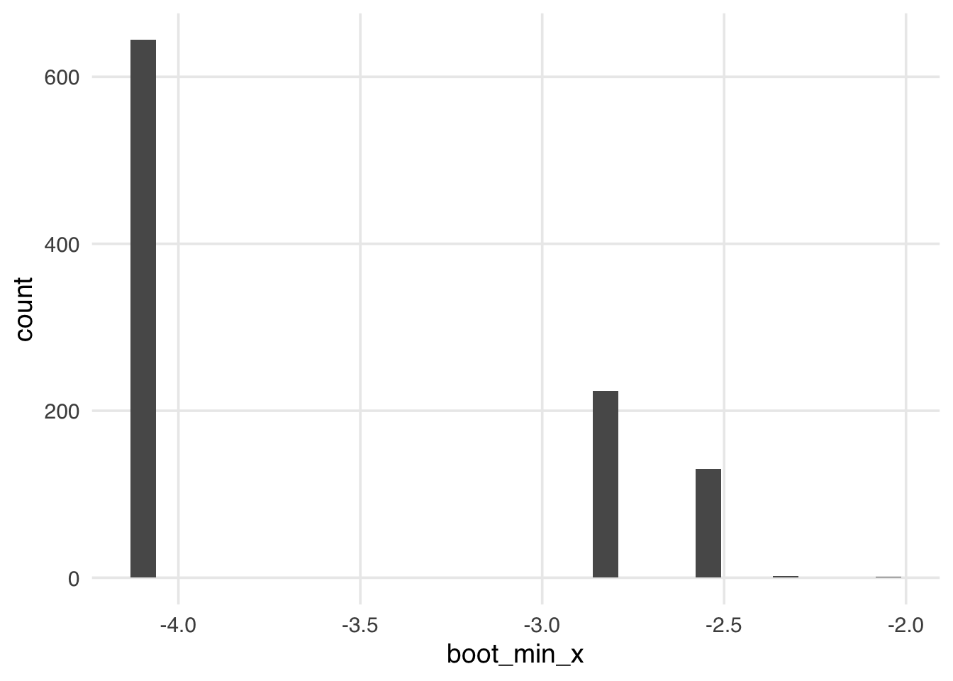

Figure A.5: The bootstrapped distribution of the sample minimum of x. The bootstrap struggles to calculate a distribution for extrema.

Other common situations where the bootstrap doesn’t work out of the box are regularized regression (like lasso regression) and data with a strong correlational structure, like time series. Often, there exists a modified version of the bootstrap that does work for a given problem. Thomas Lumley, author of the survey package and an R Core member, has an excellent summary of common situations where the bootstrap doesn’t work out of the box (and some examples of modified bootstraps that work in those scenarios) (Lumley 2017). Also see Hesterberg (2015).

Efron, Bradley. 1979. “Bootstrap Methods: Another Look at the Jackknife.” The Annals of Statistics 7 (1). https://doi.org/10.1214/aos/1176344552.

Efron, Bradley, and Robert J. Tibshirani. 1993. An Introduction to the Bootstrap. Monographs on Statistics and Applied Probability 57. Boca Raton, Florida, USA: Chapman & Hall/CRC.

Hesterberg, Tim C. 2015. “What Teachers Should Know About the Bootstrap: Resampling in the Undergraduate Statistics Curriculum.” The American Statistician 69 (4): 371–86. https://doi.org/10.1080/00031305.2015.1089789.

Lumley, Thomas. 2017. “When the Bootstrap Doesn’t Work.” Biased and Inefficient. https://notstatschat.rbind.io/2017/02/01/when-the-bootstrap-doesnt-work/.