Work-in-progress 🚧
You are reading the work-in-progress first edition of Causal Inference in R. This chapter is actively undergoing work and may be restructured or changed. It may also be incomplete.
You are reading the work-in-progress first edition of Causal Inference in R. This chapter is actively undergoing work and may be restructured or changed. It may also be incomplete.
Missing and mismeasured data are problems for most real datasets that impact all three types of analysis: description, prediction, and causal inference. As with analysis, the impact of missingness and mismeasurement is also different across all three, even when we use the same tools (like multiple imputation) to address it. At their best, missingness and mismeasurement can worsen the precision and bias of the sample; at their worst, they can create unresolvable selection bias, giving you a completely wrong answer. In this chapter, we’ll explore how bias can arise in causal analyses in the presence of missingness and mismeasurement and how to address them (if we can!).
It’s frequently been observed that causal inference can be thought of fundamentally as a missing data problem; after all, we want to compare counterfactual states, but all such states outside of the factual world are missing. Causal inference as missingness is interesting philosophically and connects methods from the two areas of statistics. Here, we’ll consider the reverse proposition: missingness and measurement error are causal inference problems.
Thus far, we’ve made a big assumption in our DAGs that the variables we’ve included are actually the variables in our data. In other words, we assume that the data is measured perfectly and completely. This assumption is almost always untrue. Let’s consider a few scenarios using causal diagrams to understand the impact of mismeasurement and missingness.
If x is partially missing but y is not, you can measure the mean of y with a higher sample size than the mean of x. However, for joint parameters, like a regression coefficient, you can only calculate the value for observations where both x and y are complete. Many tools in R, like lm(), quietly drop rows that are not complete for necessary variables by default.
Using only observation where the needed variables are all complete is sometimes called a complete-case analysis, which we’ve been doing thus far in the book.
In the TouringPlans data, most variables are complete and likely accurately measured (e.g., ticket season and historic weather are well-measured). One variable with missingness and measurement error is the actual wait times for rides. If you recall, the data relies on humans to wait in line, either consumers of the data who report their experience or people hired to wait in line to report the wait time. Thus, missingness is primarily related to whether someone is there to measure the wait time. When someone is there to measure it, it’s also likely measured with error, and that error likely depends on who the person is. For example, a visitor to Disney World estimating their wait time and submitting it to TouringPlans is likely producing a value with more error than someone paid to stay in line and count the minutes.
That said, let’s take measurement error and missingness one at a time.
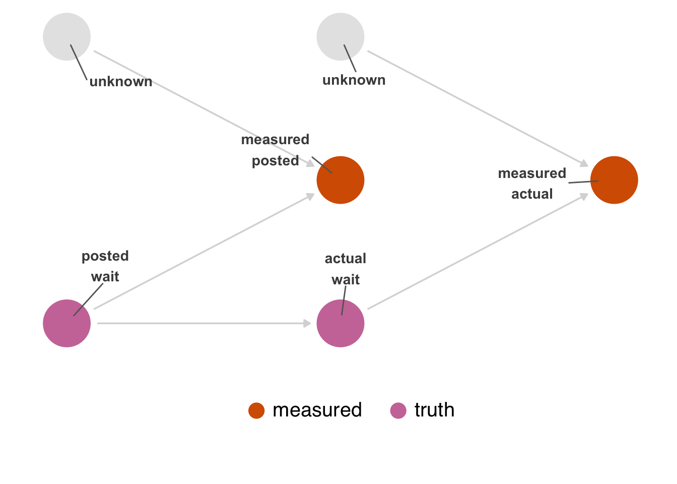
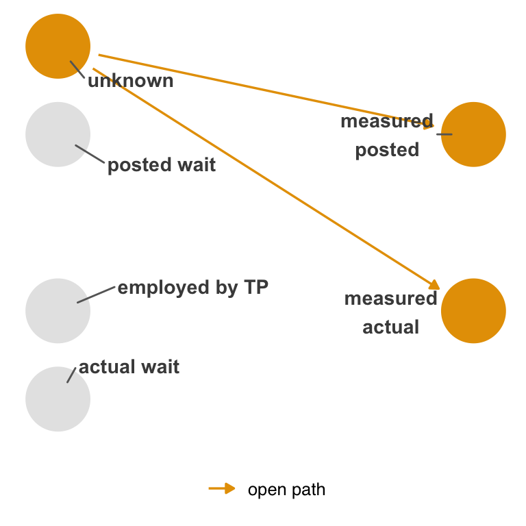
First, let’s consider measurement error. In Figure 15.1, we represent actual and posted wait times twice: the true version and the measured version. The measured versions are influenced by two variables: the real values and unknown or unmeasured factors that influence their mismeasurement. How the two wait times are mismeasured are independent of one another. For simplicity, we’ve removed the confounders from this DAG.
library(ggdag)

glyph <- function(data, params, size) {
  # data$shape <- 15
  data$size <- 5
  ggplot2::draw_key_point(data, params, size)
}

show_edge_color <- function(...) {
  list(
    theme(legend.position = "bottom"),
    ggokabeito::scale_edge_color_okabe_ito(
      name = NULL,
      breaks = ~ .x[!is.na(.x)]
    ),
    guides(color = "none")
  )
}

edges_with_aes <- function(..., edge_color = "grey85", shadow = TRUE) {
  list(
    if (shadow) {
      geom_dag_edges_link(
        data = \(.x) filter(.x, is.na(path)),
        edge_color = edge_color
      )
    },
    geom_dag_edges_link(
      aes(edge_color = path),
      data = \(.x) mutate(.x, path = if_else(is.na(to), NA, path))
    )
  )
}

ggdag2 <- function(
  .dag,
  ...,
  order = 1:9,
  seed = 1633,
  box.padding = 3.4,
  edges = geom_dag_edges_link(edge_color = "grey85")
) {
  ggplot(
    .dag,
    aes_dag(...)
  ) +
    edges +
    geom_dag_point(key_glyph = glyph) +
    geom_dag_text_repel(
      aes(label = label),
      size = 3.8,
      seed = seed,
      color = "#494949",
      box.padding = box.padding
    ) +
    ggokabeito::scale_color_okabe_ito(
      order = order,
      na.value = "grey90",
      breaks = ~ .x[!is.na(.x)]
    ) +
    theme_dag() +
    theme(legend.position = "none") +
    coord_cartesian(clip = "off")
}

add_measured <- function(.df) {
  mutate(
    .df,
    measured = case_when(
      str_detect(label, "measured") ~ "measured",
      str_detect(label, "wait") ~ "truth",
      .default = NA
    )
  )
}

add_missing <- function(.df) {
  mutate(
    .df,
    missing = case_when(
      str_detect(label, "missing") ~ "missingness indicator",
      str_detect(label, "wait") ~ "wait times",
      .default = NA
    )
  )
}

labels <- c(
  "actual" = "actual\nwait",
  "actual_star" = "measured\nactual",
  "posted" = "posted\nwait",
  "posted_star" = "measured\nposted",
  "u_posted" = "unknown",
  "u_actual" = "unknown "
)

dagify(
  actual ~ posted,
  posted_star ~ u_posted + posted,
  actual_star ~ u_actual + actual,
  coords = time_ordered_coords(),
  labels = labels,
  exposure = "posted_star",
  outcome = "actual_star"
) |>
  tidy_dagitty() |>
  add_measured() |>
  ggdag2(color = measured, order = 6:7) +
  theme(legend.position = "bottom") +
  labs(color = NULL) +
  theme(
    legend.key.spacing.x = unit(4, "points"),
    legend.key.size = unit(1, "points"),
    legend.text = element_text(
      size = rel(1.25),
      margin = margin(l = -10.5, b = 2.6)
    ),
    legend.box.margin = margin(b = 20),
    strip.text = element_blank()
  )
TouringPlans scraped the posted wait times from what Disney posts on the web. There is a plausible mechanism by which this could be mismeasured: Disney could post the wrong times online compared to what’s posted at the park, or TouringPlans could have a mistake in its data acquisition code. That said, it’s reasonable to assume this error is small.
On the other hand, actual wait times probably have a lot of measurement error. Humans have to measure this period manually, so that process has some natural error. Measurement also likely depends on whether or not the person measuring the wait time is being paid to do so. Presumably, someone entering it out of goodwill is more likely to submit an approximate wait time, and someone who is paid is more likely to be precise.
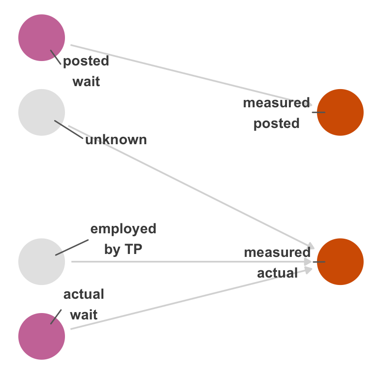
So, an updated DAG might look like Figure 15.2. This DAG describes the structural causes of measurement error in actual; notably, that structure is not connected to posted. It is easier to see if we show a null DAG with no arrow from posted to actual (Figure 15.3). Posted time is not connected to the mechanisms that cause measurement error in actual time. In other words, the bias caused by this measurement error is not due to nonexchangeability; it’s due to a numerical error in the measurement, not an open path in the causal graph. The extent of this error depends on how well the measured version correlates with the real values.
labels <- c(
  "actual" = "actual\nwait",
  "actual_star" = "measured\nactual",
  "posted" = "posted\nwait",
  "posted_star" = "measured\nposted",
  "employed" = "employed\nby TP",
  "u_actual" = "unknown"
)

dagify(
  actual ~ posted,
  posted_star ~ posted,
  actual_star ~ u_actual + actual + employed,
  coords = time_ordered_coords(),
  labels = labels
) |>
  tidy_dagitty() |>
  add_measured() |>
  ggdag2(color = measured, order = 6:7, box.padding = 3.7, seed = 123)

dagitty::dagitty(
  'dag {
actual [pos="1.000,-2.000"]
actual_star [pos="2.000,-1.000"]
employed [pos="1.000,-1.000"]
posted [pos="1.000,2.000"]
posted_star [pos="2.000,1.000"]
u_actual [pos="1.000,1.000"]
actual -> actual_star
employed -> actual_star
posted -> posted_star
u_actual -> actual_star
}'
) |>
  dag_label(labels = labels) |>
  add_measured() |>
  ggdag2(color = measured, order = 6:7, box.padding = 2.5)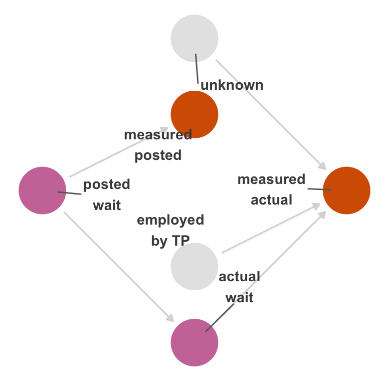
Instead of the type of nonexchangeability induced by confounding, this type of measurement bias is due to the fact that we’re analyzing the effect of posted_measured to actual_measured as a proxy for the effect of posted on actual. The correctness of the result depends entirely on how well actual_measured approximates actual. If you change your point of view to treating the measured variables as the cause and effect under study, you’ll see that we’re actually using the causal structure to approximate the study of the real variables. The measured variables in Figure 15.2 do not cause one another. However, if we calculate their relationship, they’ll be confounded by the real variables. Unusually, we’re using this confounding to approximate the relationship in the real variables. The extent to which we can do that depends on exchangeability with the exception of the real variables and the amount of independent measurement error for each variable (such as unknown here).
This is sometimes called independent, non-differential measurement error: the error is not due to structural nonexchangeability but the differences in the observed and real values for actual and posted times.
As the correlation approaches 0, measurement becomes random for the relationship under study. This often means that when variables are measured with independent measurement error, the relationship of the measured values approaches null even if there is an arrow between the true values. Here, the coefficient of x should be about 1, but as the random measurement worsens, the coefficient gets closer to 0. There’s no relationship between the randomness (u) induced by mismeasurement and y.
n <- 1000
x <- rnorm(n)
y <- x + rnorm(n)
# bad measurement of x
u <- rnorm(n)
x_measured <- 0.01 * x + u
cor(x, x_measured)
[1] -0.008004lm(y ~ x_measured)
Call:
lm(formula = y ~ x_measured)

Coefficients:
(Intercept)   x_measured
    -0.0397       0.0085
Not all random mismeasurement will bring the effect towards the null, however. For instance, for categorical variables with more than two categories, mismeasurement changes the distribution of counts of their values (this is sometimes called misclassification for categorical variables). Even in random misclassification, some of the relationships will be biased towards the null and some away from the null simply because when counts are removed from one category, they go into another. For instance, if we randomly mix up the labels "c" and "d", they average towards each other, making the coefficient for c too big and the coefficient for d too small, while the other two remain correct.
x <- sample(letters[1:5], size = n, replace = TRUE)
y <- case_when(
  x == "a" ~ 1 + rnorm(n),
  x == "b" ~ 2 + rnorm(n),
  x == "c" ~ 3 + rnorm(n),
  x == "d" ~ 4 + rnorm(n),
  x == "e" ~ 5 + rnorm(n),
)

x_measured <- if_else(
  x %in% c("c", "d"),
  sample(c("c", "d"), size = n, replace = TRUE),
  x
)

lm(y ~ x_measured)
Call:
lm(formula = y ~ x_measured)

Coefficients:
(Intercept)  x_measuredb  x_measuredc  x_measuredd
      1.145        0.857        2.442        2.455
x_measurede
      3.823
Some researchers rely on the hope that random measurement error is predictably towards the null, but this isn’t always true. See Yland et al. (2022) for more details on when this is false.
However, let’s say that a single unknown factor affects the measurement of both the posted wait time and actual wait time, as in Figure 15.4. In addition to the problem above, there’s also nonexchangeability because of confounding in the measured variables (Figure 15.5). This is called dependent, non-differential measurement error.
labels <- c(
  "actual" = "actual wait",
  "actual_star" = "measured\nactual",
  "posted" = "posted wait",
  "posted_star" = "measured\nposted",
  "employed" = "employed by TP",
  "u_actual" = "unknown"
)

depend_dag <- dagify(
  posted_star ~ posted + u_actual,
  actual_star ~ u_actual + actual + employed,
  coords = time_ordered_coords(),
  labels = labels,
  exposure = "posted_star",
  outcome = "actual_star"
)

depend_dag |>
  tidy_dagitty() |>
  add_measured() |>
  ggdag2(color = measured, order = 6:7, box.padding = 3)

depend_dag |>
  tidy_dagitty() |>
  dag_paths() |>
  ggdag2(
    color = path,
    edge_color = path,
    box.padding = 2.35,
    edges = edges_with_aes(shadow = FALSE)
  ) +
  show_edge_color()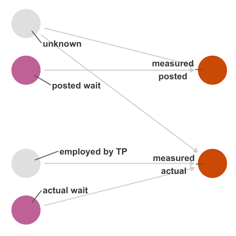
unknown to both measured variables, meaning that the way they are mismeasured is not independent. In other words, unknown is now a mutual cause of the mismeasured variables—a confounder.
unknown.
When the nonexchangeability is related to the exposure, outcome, or both, it’s called differential measurement error, which can be dependent or independent. Let’s expand Figure 15.4 to include an arrow from posted time to how actual wait time is measured, a case of dependent, differential measurement error (without the path introduced in Figure 15.4, it would be independent and differential). Figure 15.6 shows two open backdoor paths: the path via unknown and the path via posted.
labels <- c(
  "actual" = "actual wait",
  "actual_star" = "measured\nactual",
  "posted" = "posted wait",
  "posted_star" = "measured\nposted",
  "employed" = "employed by TP",
  "u_actual" = "unknown"
)

depend_dag <- dagify(
  posted_star ~ posted + u_actual,
  actual_star ~ u_actual + actual + employed + posted,
  coords = time_ordered_coords(),
  labels = labels,
  exposure = "posted_star",
  outcome = "actual_star"
)

depend_dag |>
  tidy_dagitty() |>
  dag_paths() |>
  ggdag2(
    color = path,
    edge_color = path,
    seed = 234,
    edges = edges_with_aes(edge_color = "grey90")
  ) +
  show_edge_color() +
  facet_wrap(~set) +
  theme(strip.text = element_blank())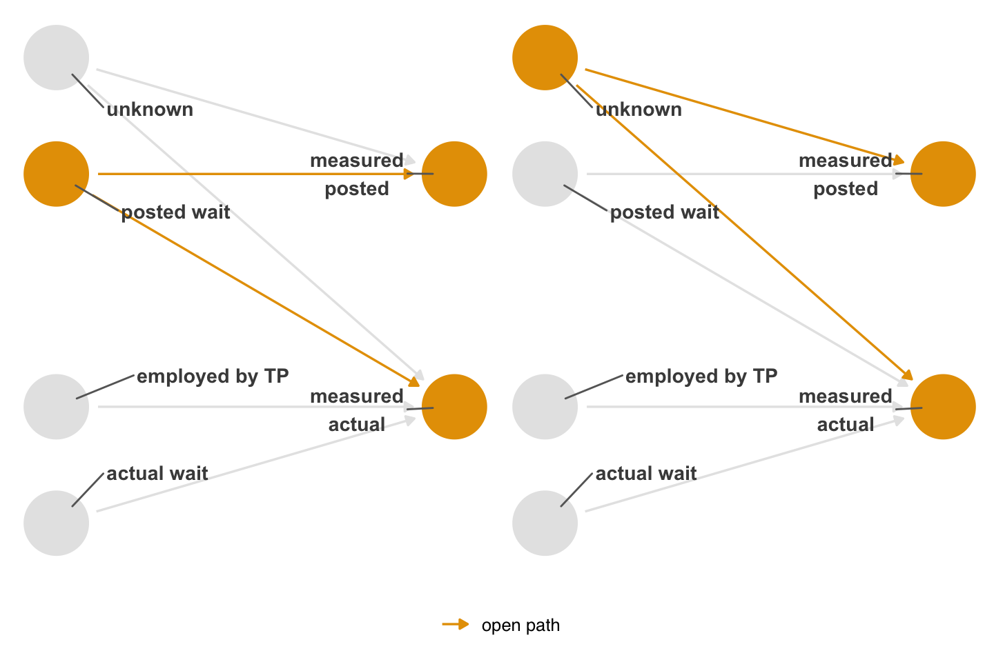
The names of the types of measurement error are conceptual. In reality, there are just two forms of bias happening: numerical inconsistency of the measured variables with their real values (independent, non-differential measurement error) and nonexchangeability (the other three types of measurement error). Whether the error is dependent or differential is based on whether the nonexchangeability involves the exposure and/or the outcome.
One inconvenience of the dependent/differential groupings is that it masks the fact that these two sources of bias can and do occur together. Often, all of these circumstances occur together (numerical inconsistency with the true values and open backdoor paths involving the exposure/outcome as well as other paths). In this case, the bias is due to both how well the measured variable correlates with the true variable and structural nonexchangeability.
In this case, posted time is unlikely to impact the measurement quality of actual time, so we can probably rule the extra arrow in Figure 15.6 out (although we’ll see below that it may affect the missingness of actual time). The measurement of posted times also probably occurs before the measurement of actual time, so there can’t be an arrow there.
The reason why we can have a situation where, for instance, the outcome affects the measurement of the exposure is that the measurement of variables may not match the time-ordering of the values they represent. An exposure may happen long before an outcome, but their measurement could happen in any order. Using values measured in time order helps avoid some types of measurement error, such as when the outcome impacts the measurement of the exposure. Either way, correctly representing occurrence and measurement in your DAG can help you identify and understand problems.
Mismeasured confounders also cause problems. Firstly, if we have a poorly measured confounder, we may not have closed the backdoor path completely, meaning there is residual confounding. Secondly, mismeasured confounders can also appear to be effect modifiers when the mismeasurement is differential with respect to the outcome. Usually, the bias from the residual confounding is worse, but there is often a small but significant interaction effect between the exposure and the mismeasured confounder, as shown in Table 15.1.
n <- 10000
set.seed(1)
confounder <- rnorm(n)
exposure <- confounder + rnorm(n)
outcome <- exposure + confounder + rnorm(n)

true_model <- lm(outcome ~ exposure * confounder)

# mismeasure confounder
confounder <- if_else(
  outcome > 0,
  confounder,
  confounder + 10 * rnorm(n)
)

mismeasured_model <- lm(outcome ~ exposure * confounder)library(gt)
library(broom)
pull_interaction <- function(mdl) {
mdl |>
tidy() |>
filter(term == "exposure:confounder") |>
mutate(
estimate = round(estimate, 3),
p.value = scales::label_pvalue()(p.value)
) |>
select(term, estimate, `p-value` = p.value)
}
map(
list("true" = true_model, "mismeasured" = mismeasured_model),
pull_interaction
) |>
list_rbind(names_to = "model") |>
gt()| model | term | estimate | p-value |
|---|---|---|---|
| true | exposure:confounder | 0.001 | 0.850 |
| mismeasured | exposure:confounder | 0.009 | <0.001 |
Above, we argued that posted wait time likely has no impact on the measurement of actual wait time. However, the posted wait time may influence the missingness of the actual wait time. If the posted wait time is high, someone may not get in the line and thus not submit an actual wait time to TouringPlans. For simplicity, we’ve removed details about measurement error and assume that the variables are well-measured and free from confounding.
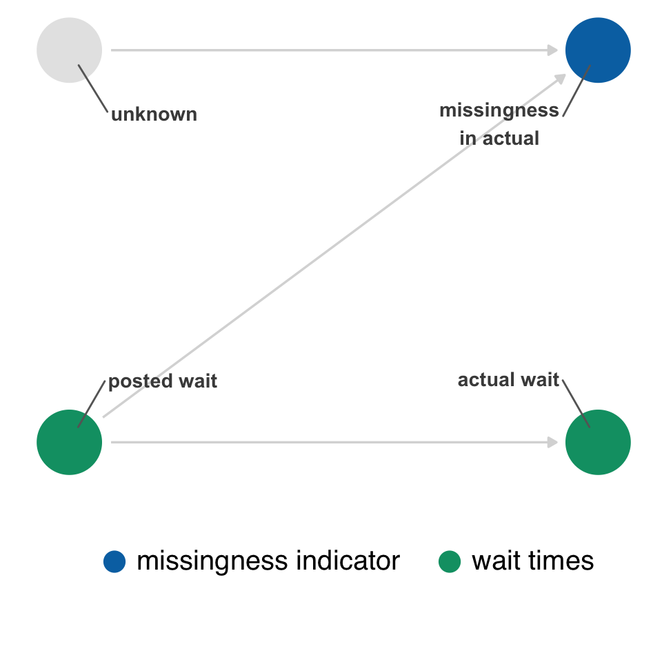
Figure 15.7 represents a slightly different situation than the DAGs in the measurement error examples. We still have two nodes for a given variable, but one represents the true values, and the other represents a missingness indicator, whether the value is missing or not. The problem is that we are inherently conditioning whether or not we observed the data. We are always conditioning on the data we actually have. In the case of missingness, we’re usually talking about conditioning on complete observations, e.g., we’re using the subset of data where all the values are complete for the variables we need. In the best case, missingness is unrelated to the causal structure of the research question, and the only impact is a reduction in sample size (and thus precision).
In Figure 15.7, though, we’re saying that the missingness of actual is related to the posted wait times and to an unknown mechanism. The unknown mechanism is random, but the mechanism related to posted wait times is not since it’s the exposure.
labels <- c(
  "actual" = "actual wait",
  "actual_missing" = "missingness\nin actual",
  "posted" = "posted wait",
  "u_actual" = "unknown"
)

missing_dag <- dagify(
  actual ~ posted,
  actual_missing ~ u_actual + posted,
  coords = time_ordered_coords(),
  labels = labels,
  exposure = "posted",
  outcome = "actual"
)

missing_dag |>
  tidy_dagitty() |>
  add_missing() |>
  ggdag2(color = missing, order = c(5, 3), box.padding = 3) +
  theme(legend.position = "bottom") +
  labs(color = NULL) +
  theme(
    legend.key.spacing.x = unit(4, "points"),
    legend.key.size = unit(1, "points"),
    legend.text = element_text(
      size = rel(1.25),
      margin = margin(l = -10.5, b = 2.6)
    ),
    legend.box.margin = margin(b = 20),
    strip.text = element_blank()
  )
However, in this simple DAG, conditioning on missingness does not open a backdoor path between actual and posted. (It does bias the relationship between unknown and posted, but we don’t care about that relationship even if we could estimate it.) The only open path in Figure 15.8 is the one from posted to actual.
missing_dag |>
  tidy_dagitty() |>
  add_missing() |>
  dag_paths(adjust_for = "actual_missing") |>
  ggdag2(
    color = path,
    edge_color = path,
    box.padding = 3,
    seed = 234,
    edges = edges_with_aes(edge_color = "grey90")
  ) +
  show_edge_color()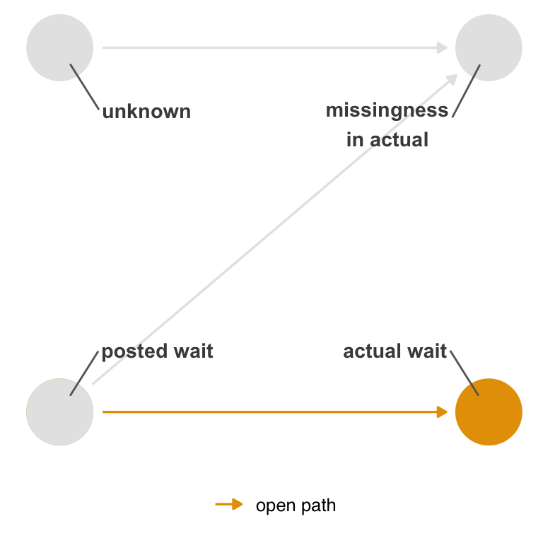
missing is a collider, stratifying on it does not open a backdoor path between the exposure and outcome.
Because we don’t have exchangeability issues, we should still be able to estimate a causal effect. Missingness still impacts the analysis, though. The causal effect in this case is recoverable; we can still estimate it without bias with complete-case analysis. However, because we’re only using observations with complete observation, we have a smaller sample size and thus reduced precision. We are also now unable to correctly estimate the mean of actual wait times because values are systematically missing by posted wait time.
Is it feasible that the missingness of actual is related to its own values? It could be that the actual wait times are so fast that a rider doesn’t have time to enter them, or it could be such a long wait that they decide to get out of line. Figure 15.9 depicts a relationship like this.
When missingness is collider, conditioning on it may induce bias. In this case, whether or not actual wait times were measured is a descendant of both the actual and posted wait times. Conditioning on it opens a backdoor path, creating nonexchangeability, as in Figure 15.10. In this case, there is no way to close the backdoor paths opened by conditioning on missingness.
labels <- c(
  "actual" = "actual wait",
  "actual_missing" = "missingness\nin actual",
  "posted" = "posted wait",
  "u_actual" = "unknown"
)

missing_dag <- dagify(
  actual ~ posted,
  actual_missing ~ u_actual + actual + posted,
  coords = time_ordered_coords(),
  labels = labels,
  exposure = "posted",
  outcome = "actual"
)

missing_dag |>
  tidy_dagitty() |>
  add_missing() |>
  ggdag2(color = missing, order = c(5, 3))

missing_dag |>
  tidy_dagitty() |>
  add_missing() |>
  dag_paths(adjust_for = "actual_missing") |>
  ggdag2(
    color = path,
    edge_color = path,
    seed = 234,
    edges = edges_with_aes(edge_color = "grey90")
  ) +
  show_edge_color() +
  facet_wrap(~set) +
  expand_plot(expand_x = expansion(c(0.2, 0.2))) +
  theme(strip.text = element_blank())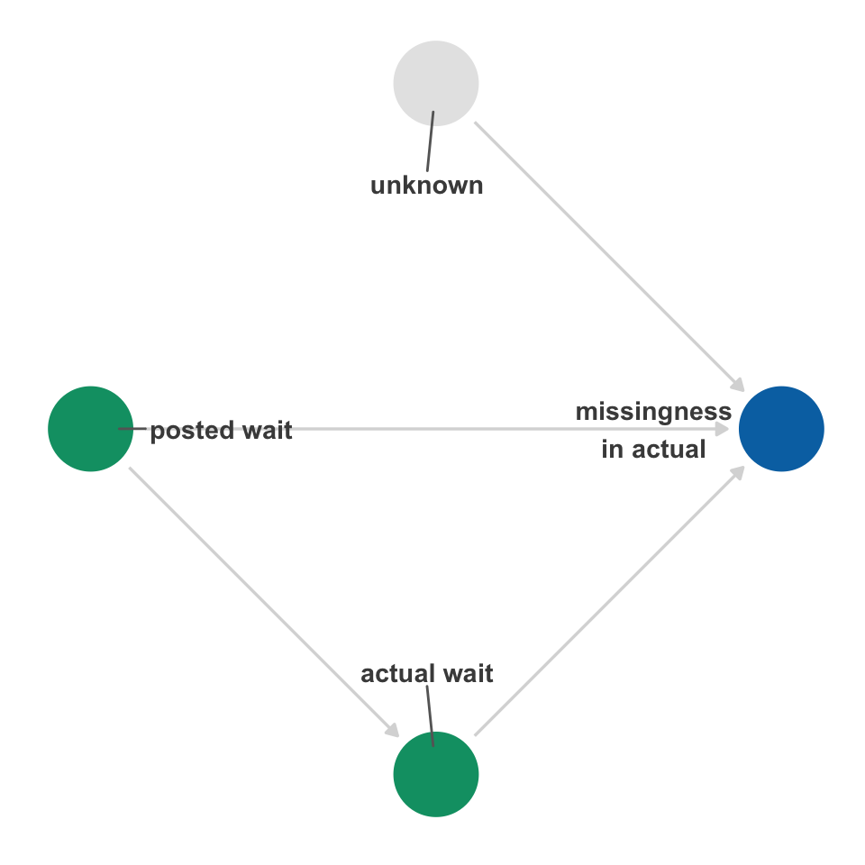
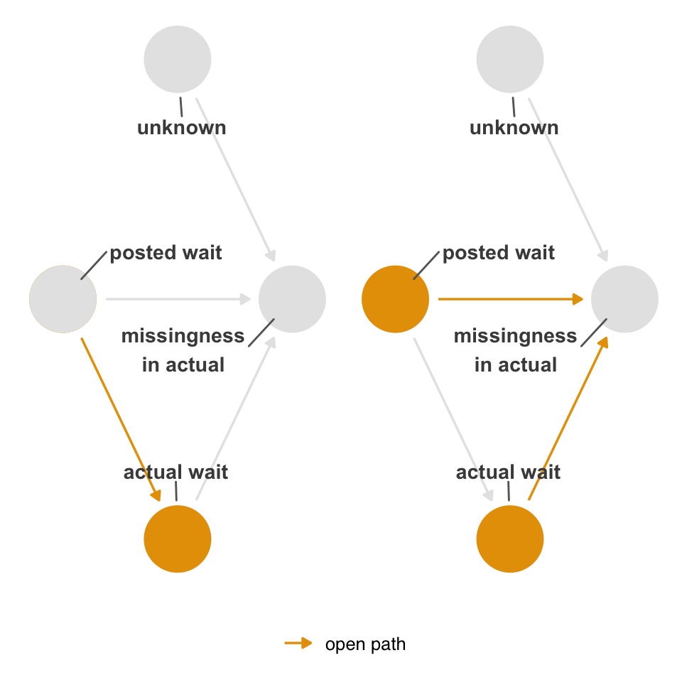
What effects we can recover is more complicated than determining backdoor paths alone. When there are no backdoor paths, we can calculate the causal effect, but we may not be able to calculate other statistics like the mean of the exposure or outcome. When conditioning on missingness opens a backdoor path, sometimes we can close it (and thus estimate a causal effect), and sometimes we can’t.
Consider the DAGs in Figure 15.11, where a is actual, p is posted, u is unknown, and m is missing. Each of the DAGs represents a simple but differing structure of missingness.
library(patchwork)

define_dag <- function(..., tag, title) {
  dagify(
    ...,
    coords = time_ordered_coords(),
    exposure = "p",
    outcome = "a"
  ) |>
    ggdag(size = 0.7) +
    labs(title = paste0(tag, ": ", title)) +
    theme_dag() +
    theme(plot.title = element_text(size = 12)) +
    expand_plot(expansion(c(0.4, 0.4)), expansion(c(0.4, 0.4)))
}

dag_1 <- define_dag(
  a ~ p,
  m ~ u,
  tag = "1",
  title = "`actual` is missing"
)

dag_2 <- define_dag(
  a ~ p,
  m ~ u + p,
  tag = "2",
  title = "`actual` is missing"
)

dag_3 <- define_dag(
  a ~ p,
  m ~ u + a,
  tag = "3",
  title = "`actual` is missing"
)

dag_4 <- define_dag(
  a ~ p,
  m ~ u + p,
  tag = "4",
  title = "`posted` is missing"
)

dag_5 <- define_dag(
  a ~ p,
  m ~ u + a,
  tag = "5",
  title = "`posted` is missing"
)

(dag_1 + dag_2 + dag_3) / (plot_spacer() + dag_4 + dag_5)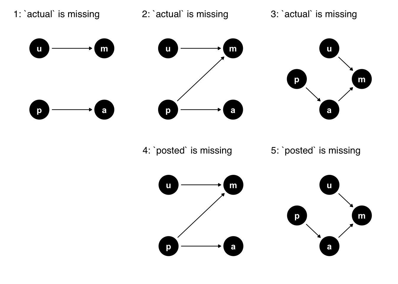
a is actual, p is posted, u is unknown, and m is missing. Each DAG represents a slightly different missingness mechanism. In DAGs 1-3, the actual wait time values have missingness; in DAGs 4-5, some posted wait times are missing. The causal structure of missingness impacts what we can estimate.
Figure 15.12 presents the mean of posted and actual and the estimated causal effect of posted on actual for data simulated from these DAGs. Without any missingness, of course, we can estimate all three. For DAG 1, we can also estimate all three, but because of missingness, we have a reduced sample size and, thus, worse precision. For DAG 2, we can calculate the mean of posted and the causal effect but not the mean of actual. For DAG 3, we also can’t calculate the causal effect. In DAG 4, we can calculate the mean of actual and the causal effect but not the mean of posted, and in DAG 5, we can calculate the mean of actual, but that’s it.
set.seed(123)
posted <- rnorm(365, mean = 30, sd = 5)
# create an effect where an hour of posted time creates 50 min of actual time
coef <- 50 / 60
actual <- coef * posted + rnorm(365, mean = 0, sd = 2)

posted_60 <- posted / 60
missing_dag_1 <- rbinom(365, 1, 0.3) |>
  as.logical()
missing_dag_2 <- if_else(posted_60 > 0.50, rbinom(365, 1, 0.95), 0) |>
  as.logical()
missing_dag_3 <- if_else(actual > 22, rbinom(365, 1, 0.99), 0) |>
  as.logical()
# the same structure, but it's `posted` that gets the resulting missingness
missing_dag_4 <- missing_dag_2
missing_dag_5 <- missing_dag_3

fit_stats <- function(
  dag,
  actual,
  posted_60,
  missing_by = NULL,
  missing_for = "actual"
) {
  if (!is.null(missing_by) && missing_for == "actual") {
    actual[missing_by] <- NA
  }

  if (!is.null(missing_by) && missing_for == "posted") {
    posted_60[missing_by] <- NA
  }

  t_actual <- t.test(actual)
  t_posted <- t.test(posted_60 * 60)
  mdl <- lm(actual ~ posted_60)
  mdl_confints <- confint(mdl)

  tibble(
    dag = dag,
    mean_actual_estimate = as.numeric(t_actual$estimate),
    mean_actual_lower = t_actual$conf.int[[1]],
    mean_actual_upper = t_actual$conf.int[[2]],
    mean_posted_estimate = as.numeric(t_posted$estimate),
    mean_posted_lower = t_posted$conf.int[[1]],
    mean_posted_upper = t_posted$conf.int[[2]],
    coef_60_estimate = coefficients(mdl)[["posted_60"]],
    coef_60_lower = mdl_confints[2, 1],
    coef_60_upper = mdl_confints[2, 2]
  ) |>
    pivot_longer(
      cols = -dag,
      names_to = c("stat", ".value"),
      names_pattern = "^(.*)_(estimate|lower|upper)$"
    )
}

dag_stats <- bind_rows(
  fit_stats("No missingness", actual, posted_60),
  fit_stats("DAG 1", actual, posted_60, missing_by = missing_dag_1),
  fit_stats("DAG 2", actual, posted_60, missing_by = missing_dag_2),
  fit_stats("DAG 3", actual, posted_60, missing_by = missing_dag_3),
  fit_stats(
    "DAG 4",
    actual,
    posted_60,
    missing_by = missing_dag_4,
    missing_for = "posted"
  ),
  fit_stats(
    "DAG 5",
    actual,
    posted_60,
    missing_by = missing_dag_5,
    missing_for = "posted"
  ),
)

dag_stats |>
  mutate(
    true_value = if_else(
      dag == "No missingness",
      "True value",
      "Observed value"
    ),
    dag = factor(dag, levels = c(paste("DAG", 5:1), "No missingness")),
    stat = factor(
      stat,
      levels = c("mean_posted", "mean_actual", "coef_60"),
      labels = c("Mean of Posted", "Mean of Actual", "Causal effect")
    )
  ) |>
  ggplot(aes(color = true_value)) +
  geom_point(aes(estimate, dag)) +
  geom_segment(aes(
    x = lower,
    xend = upper,
    y = dag,
    yend = dag,
    group = stat
  )) +
  facet_wrap(~stat, scales = "free_x") +
  labs(y = NULL, color = NULL)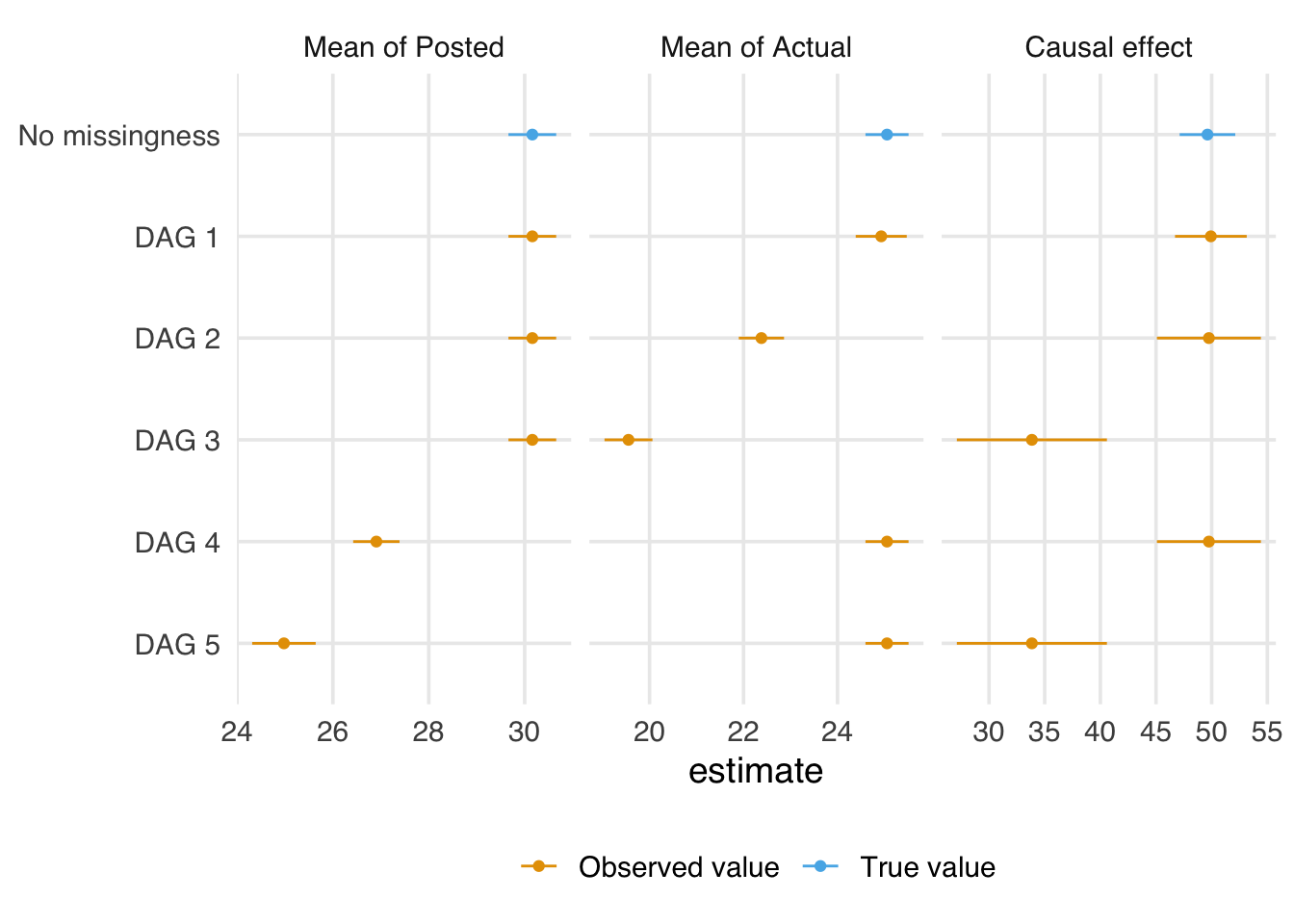
See Moreno-Betancur et al. (2018) for a comprehensive overview of what effects are recoverable from different structures of missingness.
As in measurement error, the confounders in the causal model may also contribute to the missingness of actual wait time, such as if season or temperature influences whether TouringPlans sends someone in to do a measurement. In these data, all the confounders are observed, but missingness in confounders can cause both residual confounding and selection bias from stratification on complete cases.
In the grand tradition of statisticians being bad at naming things, you’ll also commonly see missingness discussed in terms of missing completely at random, missing at random, and missing not at random.
In the case of causal models, we can explain these ideas by the causal structure of missingness and the availability of variables and values related to that structure in your data.
x are more likely to be missing in x. We don’t have that information because, by definition, it’s missing.These terms don’t always tell you what to do next, so we’ll avoid them in favor of explicitly describing the missingness generation process.
Is measurement error missingness because we’re missing the true value? Is missingness measurement error, because we’ve badly mismeasured some values as NA? We’ve presented the two problems using different structures, where measurement error is represented by calculating the causal effects of proxy variables, and missingness is represented by calculating the causal effects of the true variables conditional on missingness. These two structures better illuminate the biases that emerge from the two situations. That said, it can also be helpful to think of them from the other perspective. For instance, thinking about measurement error as a missingness problem allows you to use techniques like multiple imputation to address it. Of course, we often do both because data are missing for some observations and observed but mismeasured for others.
Now, let’s discuss some analytic techniques for addressing measurement error and missingness to correct for both the numerical issues and structural nonexchangeability we see in these DAGs. In Chapter 16, we’ll also discuss sensitivity analyses for missingness and measurement error.
Sometimes, you have a well-measured version of a variable for a subset of observations and a version with more measurement error for a more significant proportion of the dataset. Sometimes people call this a validation set. When this is the case, you can use a simple approach called regression calibration to predict the value of the well-measured version for more observations in the dataset. This technique’s name refers to the fact that you’re recalibrating the variable that you’ve observed more of, given the subset of values you have for the well-measured version. But other than that, it’s just a prediction model that includes the version of the variable you have more observations of and other variables you find essential to the measurement process.
As we know, the actual wait times have a lot of missingness. What if we considered posted wait times a proxy for actual wait times? In this case, we could redo the analysis of Extra Magic Morning’s effect on the calibrated version of actual wait times.
First, we’ll fit a model to predict wait_minutes_actual_avg using wait_minutes_posted_avg. Then, instead of using wait_minutes_posted_avg we’ll use the calibrated value from that model in it’s place.
When fitting regression calibration models, it is crucial to include all variables that will be in subsequent models in the same form they will be there (for example, if we have a confounder in our final model that is fit using a spline, we need this same confounder, fit using a spline, in our calibration model).
library(splines)
library(touringplans)
library(broom)

calib_model <- lm(
  wait_minutes_actual_avg ~
    wait_minutes_posted_avg *
    wait_hour +
    park_extra_magic_morning +
    park_temperature_high +
    park_close +
    park_ticket_season,
  data = seven_dwarfs_train_2018
)

seven_dwarves_calib <- calib_model |>
  augment(newdata = seven_dwarfs_train_2018) |>
  rename(wait_minutes_posted_calib = .fitted)
Fitting this model with the IPW estimator results in an effect of 4.91, marginally attenuated compared to the value we saw when using the uncalibrated wait_minutes_posted_avg in Chapter 11.
Another approach could be to impute the values. Where wait_minutes_actual_avg is available, we’ll use that. If it’s NA, we’ll use the calibrated value. In practice, this uses the same calibration model as above, but instead of giving the calibrated values to all observations, we only impute them for the observations missing in the validation set. This method is sometimes called regression imputation or deterministic imputation. It is deterministic in the sense that we are just giving every observation with missing data a single predicted value and treating it as fixed rather than adding any variability (we’ll see a stocastic imptuation method next, where we introduce some variability).
seven_dwarves_reg_impute <- calib_model |>
  augment(newdata = seven_dwarfs_train_2018) |>
  rename(wait_minutes_actual_impute = .fitted) |>
  # fill in real values where they exist
  mutate(
    wait_minutes_actual_impute = coalesce(
      wait_minutes_actual_avg,
      wait_minutes_actual_impute
    )
  )
Fitting this model with the IPW estimator results in an effect of 6.49.
The regression calibration model introduces uncertainty into the estimates of calibrated variables. Be sure to include the fitting of this model in your bootstrap to get the correct standard errors when performing regression calibration or imputation.
Regression calibration provides a straightforward way to address measurement error and missingness by predicting values with a single model and plugging those predictions into the analysis. However, this plug-in approach is generally inefficient. If we correctly estimate uncertainty (for example, by bootstrapping both the calibration and outcome models), we often end up with wide confidence intervals, reflecting the fact that we’ve relied on a single imputed value.
Multiple imputation (MI) is an often more efficient alternative. Instead of producing one “best guess” for the missing value, MI draws predicted values from a distribution, capturing the uncertainty inherent in the missing data. This process allows for better estimates of both summary statistics (like the mean of the imputed variable) and downstream conditional effects (like treatment effects when the imputed variable appears in the outcome model). Through this process, we will generate multiple imputed datasets. The default is often 5, but if a large portion of your data is missing, more imputations may be necessary to achieve stable results. A common rule of thumb is that the number of imputations should roughly match the percentage of incomplete cases.
There are a few critical modeling considerations when using MI in causal analyses:
In a typical causal analysis, we proceed as follows:
After performing the analysis separately on each of the \(m\) imputed datasets:
Let:
Then the total variance is:
\[ T = \bar{U} + \left(1 + \frac{1}{m}\right) B \]
The standard error of the pooled estimate is \(\sqrt{T}\) and this can be used to construct confidence intervals or perform hypothesis testing.
This approach accounts for uncertainty in both the imputation and the treatment effect estimation steps. It is particularly helpful when missingness affects variables involved in the treatment assignment or outcome processes, cases where complete-case analysis or single imputation can yield biased or inefficient estimates.
In practice, multiple imputation is often implemented using the MICE (Multivariate Imputation by Chained Equations) algorithm, which iteratively imputes each variable with missing values using models conditional on the others. In R, we often use the mice package to implement the imputation.
Let’s use the same example as above, but rather than just performing a single regression imputation, we will perform the stochastic (multiple) imputation 10 times. First, we need to impute our data.
library(mice)

seven_dwarfs_to_impute_data <- seven_dwarfs_train_2018 |>
  mutate(park_ticket_season = as.factor(park_ticket_season)) |>
  select(
    park_date,
    wait_minutes_actual_avg,
    wait_minutes_posted_avg,
    wait_hour,
    park_temperature_high,
    park_close,
    park_ticket_season,
    park_extra_magic_morning
  )

predictor_matrix <- make.predictorMatrix(seven_dwarfs_to_impute_data)

# remove park date from imputation models
predictor_matrix[, 1] <- 0

# Impute data
seven_dwarfs_mi <- mice(
  seven_dwarfs_to_impute_data,
  m = 10, # we are doing 10 imputations
  predictorMatrix = predictor_matrix,
  method = "pmm", # predictive mean matching
  seed = 1,
  print = FALSE
)
Then we can collect our imputed datasets into a list using the complete function:
seven_dwarfs_mi_data <- complete(seven_dwarfs_mi, action = "all")Finally, let’s write a functcion to fit the IPW effect across these datasets. We want to preserve the treatment effect as well as the standard error for applying Rubin’s Rules.
fit_ipw_effect <- function(
  .fmla,
  .data = seven_dwarfs,
  .trt = "park_extra_magic_morning",
  .outcome_fmla = wait_minutes_posted_calib ~ park_extra_magic_morning
) {
  .trt_var <- rlang::ensym(.trt)

  # fit propensity score model
  propensity_model <- glm(
    .fmla,
    data = .data,
    family = binomial()
  )

  # calculate ATE weights
  .df <- propensity_model |>
    augment(type.predict = "response", data = .data) |>
    mutate(w_ate = wt_ate(.fitted, !!.trt_var, exposure_type = "binary"))

  # fit outcome model
  outcome_model <- lm(.outcome_fmla, data = .df, weights = w_ate)

  # fit ipw effect
  ipw_output <- ipw(propensity_model, outcome_model, .df)
  return(c(
    estimate = ipw_output$estimates$estimate,
    std.err = ipw_output$estimates$std.err
  ))
}
effect_mi_all <- map(
seven_dwarfs_mi_data,
~ fit_ipw_effect(
park_extra_magic_morning ~ park_temperature_high +
park_close +
park_ticket_season,
.outcome_fmla = wait_minutes_actual_avg ~ park_extra_magic_morning,
.data = .x |> filter(wait_hour == 9)
)
) |>
bind_rows()Now we have a data frame with the estimated effect within each imputed dataset along with the standard error.
effect_mi_all# A tibble: 10 × 2
estimate std.err
<dbl> <dbl>
1 6.24 4.61
2 -1.43 3.63
3 11.5 5.27
4 10.6 5.19
5 -1.96 4.07
6 1.36 4.18
7 -2.30 3.60
8 7.20 6.06
9 7.92 4.92
10 2.98 3.86To get the final effect, we are going to average the estimate column and to get the appropriate standard errors, we will apply Rubin’s Rules (see Tip 15.1 for details).
effect_mi_all |>
  summarise(
    effect_mi = mean(estimate), # pooled estimate
    u_bar = mean(std.err^2), # average within-imputation variance
    b = var(estimate), # between-imputation variance
    t_var = u_bar + (1 + 1 / n()) * b, # total variance
    se_mi = sqrt(t_var) # pooled standard error
  ) |>
  select(effect_mi, se_mi)
# A tibble: 1 × 2
effect_mi se_mi
<dbl> <dbl>
1 4.21 7.14Again, this effect is attenuated compared to what we saw in Chapter 11 (although the standard error is quite large, so the differences may not be meaningful).
The effects of missingness on results and the impact of complete case analyses and multiple imputation can be deeply unintuitive. When you add measurement error and other types of bias, it can be nearly impossible to reason about. A partial solution to this problem is to offload some of the reasoning from your brain into the computer.
We recommend writing down the causal mechanisms you think are involved in your research question and then using simulation to probe different strategies.
As with our general suggestion about DAGs, if you are unsure about the correct DAG, you should check to see how these results differ depending on the specification.