Work-in-progress 🚧
You are reading the work-in-progress first edition of Causal Inference in R. This chapter is actively undergoing work and may be restructured or changed. It may also be incomplete.
You are reading the work-in-progress first edition of Causal Inference in R. This chapter is actively undergoing work and may be restructured or changed. It may also be incomplete.
Because many of the assumptions of causal inference are unverifiable, it’s reasonable to be concerned about the validity of your results. In this chapter, we’ll provide some ways to probe our assumptions and results for strengths and weaknesses. We’ll explore two main ways to do so: exploring the logical implications of the causal question and related DAGs and using mathematical techniques to quantify how different our results would be under other circumstances, such as in the presence of unmeasured confounding. These approaches are known as sensitivity analyses: How sensitive is our result to conditions other than those laid out in our assumptions and analysis?
Let’s start with where we began the modeling process: creating causal diagrams. Because DAGs encode the assumptions on which we base our analysis, they are natural points of critique for both others and ourselves.
The same mathematical underpinnings of DAGs that allow us to to query them for things like adjustment sets also allow us to query other implications of DAGs. One of the simplest is that if your DAG is correct and your data are well-measured, any valid adjustment set should result in an unbiased estimate of the causal effect. Let’s consider the DAG we introduced in Figure 7.2.
coord_dag <- list(
  x = c(park_ticket_season = 0, park_close = 0, park_temperature_high = -1, park_extra_magic_morning = 1, wait_minutes_posted_avg = 2),
  y = c(park_ticket_season = -1, park_close = 1, park_temperature_high = 0, park_extra_magic_morning = 0, wait_minutes_posted_avg = 0)
)

labels <- c(
  park_extra_magic_morning = "Extra Magic\nMorning",
  wait_minutes_posted_avg = "Average\nwait",
  park_ticket_season = "Ticket\nSeason",
  park_temperature_high = "Historic high\ntemperature",
  park_close = "Time park\nclosed"
)

emm_wait_dag <- dagify(
  wait_minutes_posted_avg ~ park_extra_magic_morning + park_close + park_ticket_season + park_temperature_high,
  park_extra_magic_morning ~ park_temperature_high + park_close + park_ticket_season,
  coords = coord_dag,
  labels = labels,
  exposure = "park_extra_magic_morning",
  outcome = "wait_minutes_posted_avg"
)

curvatures <- rep(0, 7)
curvatures[5] <- .3

emm_wait_dag |>
  tidy_dagitty() |>
  node_status() |>
  ggplot(
    aes(x, y, xend = xend, yend = yend, color = status)
  ) +
  geom_dag_edges_arc(curvature = curvatures, edge_color = "grey80") +
  geom_dag_point() +
  geom_dag_text_repel(aes(label = label), size = 3.8, seed = 1630, color = "#494949") +
  scale_color_okabe_ito(na.value = "grey90") +
  theme_dag() +
  theme(legend.position = "none") +
  coord_cartesian(clip = "off") +
  scale_x_continuous(
    limits = c(-1.25, 2.25),
    breaks = c(-1, 0, 1, 2)
  )
In Figure 16.1, there’s only one adjustment set because all three confounders represent independent backdoor paths. Let’s say, though, that we had used Figure 16.2 instead, which is missing arrows from the park close time and historical temperature to whether there was an Extra Magic Morning.
emm_wait_dag_missing <- dagify(
  wait_minutes_posted_avg ~ park_extra_magic_morning + park_close + park_ticket_season + park_temperature_high,
  park_extra_magic_morning ~ park_ticket_season,
  coords = coord_dag,
  labels = labels,
  exposure = "park_extra_magic_morning",
  outcome = "wait_minutes_posted_avg"
)

# produces below:
# park_ticket_season, park_close + park_ticket_season, park_temperature_high + park_ticket_season, or park_close + park_temperature_high + park_ticket_season
adj_sets <- unclass(dagitty::adjustmentSets(emm_wait_dag_missing, type = "all")) |>
  map_chr(\(.x) glue::glue('{unlist(glue::glue_collapse(.x, sep = " + "))}')) |>
  glue::glue_collapse(sep = ", ", last = ", or ")

curvatures <- rep(0, 5)
curvatures[3] <- .3

emm_wait_dag_missing |>
  tidy_dagitty() |>
  node_status() |>
  ggplot(
    aes(x, y, xend = xend, yend = yend, color = status)
  ) +
  geom_dag_edges_arc(curvature = curvatures, edge_color = "grey80") +
  geom_dag_point() +
  geom_dag_text_repel(aes(label = label), size = 3.8, seed = 1630, color = "#494949") +
  scale_color_okabe_ito(na.value = "grey90") +
  theme_dag() +
  theme(legend.position = "none") +
  coord_cartesian(clip = "off") +
  scale_x_continuous(
    limits = c(-1.25, 2.25),
    breaks = c(-1, 0, 1, 2)
)Now there are 4 potential adjustment sets: park_ticket_season, park_close + park_ticket_season, park_temperature_high + park_ticket_season, or park_close + park_temperature_high + park_ticket_season. Table 16.1 presents the IPW estimates for each adjustment set. The effects are quite different. Some slight variation in the estimates is expected since they are estimated using different variables that may not be measured perfectly; if this DAG were right, however, we should see them much more closely aligned than this. In particular, there seems to be a 3-minute difference between the models with and without park close time. The difference in these results implies that there is something off about the causal structure we specified.
seven_dwarfs <- touringplans::seven_dwarfs_train_2018 |>
  filter(wait_hour == 9)

# we'll use `.data` and `.trt` later
fit_ipw_effect <- function(.fmla, .data = seven_dwarfs, .trt = "park_extra_magic_morning", .outcome_fmla = wait_minutes_posted_avg ~ park_extra_magic_morning) {
  .trt_var <- rlang::ensym(.trt)

  # fit propensity score model
  propensity_model <- glm(
    .fmla,
    data = .data,
    family = binomial()
  )

  # calculate ATE weights
  .df <- propensity_model |>
    augment(type.predict = "response", data = .data) |>
    mutate(w_ate = wt_ate(.fitted, !!.trt_var, exposure_type = "binary"))

  # fit ipw model
  lm(.outcome_fmla, data = .df, weights = w_ate) |>
    tidy() |>
    filter(term == .trt) |>
    pull(estimate)
}

effects <- list(
  park_extra_magic_morning ~ park_ticket_season,
  park_extra_magic_morning ~ park_close + park_ticket_season,
  park_extra_magic_morning ~ park_temperature_high + park_ticket_season,
  park_extra_magic_morning ~ park_temperature_high +
    park_close + park_ticket_season
) |>
  map_dbl(fit_ipw_effect)

tibble(
  `Adjustment Set` = c(
    "Ticket season",
    "Close time, ticket season",
    "Historic temperature, ticket season",
    "Historic temperature, close time, ticket season"
  ),
  ATE = effects
) |>
  arrange(desc(ATE)) |>
gt()| Adjustment Set | ATE |
|---|---|
| Close time, ticket season | 6.579 |
| Historic temperature, close time, ticket season | 6.199 |
| Ticket season | 4.114 |
| Historic temperature, ticket season | 3.627 |
Alternate adjustment sets are a way of probing the logical implications of your DAG: if it’s correct, there could be many ways to account for the open backdoor paths correctly. The reverse is also true: the causal structure of your research question also implies relationships that should be null. One way that researchers take advantage of this implication is through negative controls. A negative control is either an exposure (negative exposure control) or outcome (negative outcome control) similar to your question in as many ways as possible, except that there shouldn’t be a causal effect. Lipsitch, Tchetgen Tchetgen, and Cohen (2010) describe negative controls for observational research. In their article, they reference standard controls in bench science. In a lab experiment, any of these actions should lead to a null effect:
There’s nothing unique to lab work here; these scientists merely probe the logical implications of their understanding and hypotheses. To find a good negative control, you usually need to extend your DAG to include more of the causal structure surrounding your question. Let’s look at some examples.
First, we’ll look at a negative exposure control. If Extra Magic Mornings really cause an increase in wait time, it stands to reason that this effect is time-limited. In other words, there should be some period after which the effect of Extra Magic Morning dissipates. Let’s call today i and the previous day i - n, where n is the number of days before the outcome that the negative exposure control occurs. First, let’s explore n = 63, e.g., whether or not there was an Extra Magic Morning nine weeks ago. That is a pretty reasonable starting point: it’s unlikely that the effect on wait time would still be present 63 days later. This analysis is an example of leaving out an essential ingredient: we waited too long for this to be a realistic cause. Any remaining effect is likely due to residual confounding.
Let’s look at a DAG to visualize this situation. In Figure 16.3, we’ve added an identical layer to our original one: now there are two Extra Magic Mornings: one for day i and one for day i - 63. Similarly, there are two versions of the confounders for each day. One crucial detail in this DAG is that we’re assuming that there is an effect of day i - 63’s Extra Magic Morning on day i’s; whether or not there is an Extra Magic Morning one day likely affects whether or not it happens on another day. The decision about where to place them across the year is not random. If this is true, we would expect an effect: the indirect effect via day i’s Extra Magic Morning status. To get a valid negative control, we need to inactivate this effect, which we can do statistically by controlling for day i’s Extra Magic Morning status. So, given the DAG, our adjustment set is any combination of the confounders (as long as we have at least one version of each) and day i’s Extra Magic Morning (suppressing the indirect effect).
labels <- c(
  x63 = "Extra Magic\nMorning (i-63)",
  x = "Extra Magic\nMorning (i)",
  y = "Average\nwait",
  season = "Ticket\nSeason",
  weather = "Historic\nhigh\ntemperature",
  close = "Time park\nclosed (i)",
  season63 = "Ticket Season\n(i-63)",
  weather63 = "Historic\nhigh\ntemperature\n(i-63)",
  close63 = "Time park\nclosed (i-63)"
)

dagify(
  y ~ x + close + season + weather,
  x ~ weather + close + season + x63,
  x63 ~ weather63 + close63 + season63,
  weather ~ weather63,
  close ~ close63,
  season ~ season63,
  coords = time_ordered_coords(),
  labels = labels,
  exposure = "x63",
  outcome = "y"
) |>
  tidy_dagitty() |>
  node_status() |>
  ggplot(
    aes(x, y, xend = xend, yend = yend, color = status)
  ) +
  geom_dag_edges_link(edge_color = "grey80") +
  geom_dag_point() +
  geom_dag_text_repel(aes(label = label), size = 3.8, color = "#494949") +
  scale_color_okabe_ito(na.value = "grey90") +
  theme_dag() +
  theme(legend.position = "none") +
  coord_cartesian(clip = "off")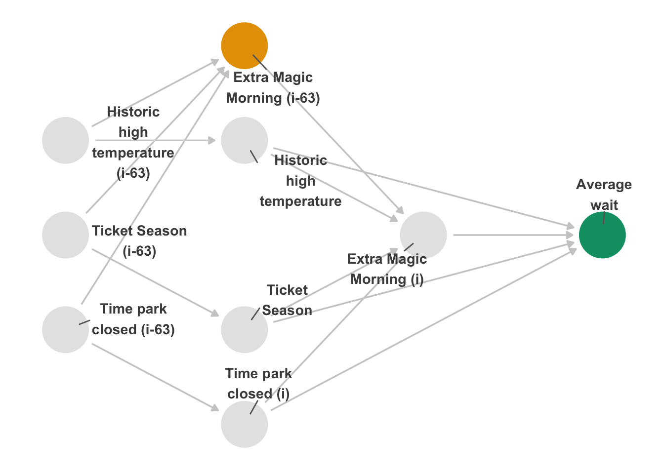
i - 63.
Since the exposure is on day i - 63, we prefer to control for the confounders related to that day, so we’ll use the i - 63 versions. We’ll use lag() from dplyr to get those variables.
n_days_lag <- 63
distinct_emm <- seven_dwarfs_train_2018 |>
  filter(wait_hour == 9) |>
  arrange(park_date) |>
  transmute(
    park_date,
    prev_park_extra_magic_morning = lag(park_extra_magic_morning, n = n_days_lag),
    prev_park_temperature_high = lag(park_temperature_high, n = n_days_lag),
    prev_park_close = lag(park_close, n = n_days_lag),
    prev_park_ticket_season = lag(park_ticket_season, n = n_days_lag)
  )

seven_dwarfs_train_2018_lag <- seven_dwarfs_train_2018 |>
  filter(wait_hour == 9) |>
  left_join(distinct_emm, by = "park_date") |>
  drop_na(prev_park_extra_magic_morning)
When we use these data for the IPW effect, we get -0.93 minutes, much closer to null than we found on day i. Let’s take a look at the effect over time. While there might be a lingering effect of Extra Magic Mornings for a little while (say, the span of an average trip to Disney World), it should quickly approach null. However, in Figure 16.4, we see that, while it eventually approaches null, there is quite a bit of lingering effect. If these results are accurate, it implies that we have some residual confounding in our effect.
coefs <- purrr::map_dbl(1:63, calculate_coef)

ggplot(tibble(coefs = coefs, x = 1:63), aes(x = x, y = coefs)) +
  geom_hline(yintercept = 0) +
  geom_point() +
  geom_smooth(se = FALSE) +
  labs(y = "difference in wait times (minutes)\n on day (i) for EMM on day (i - n)", x = "day (i - n)")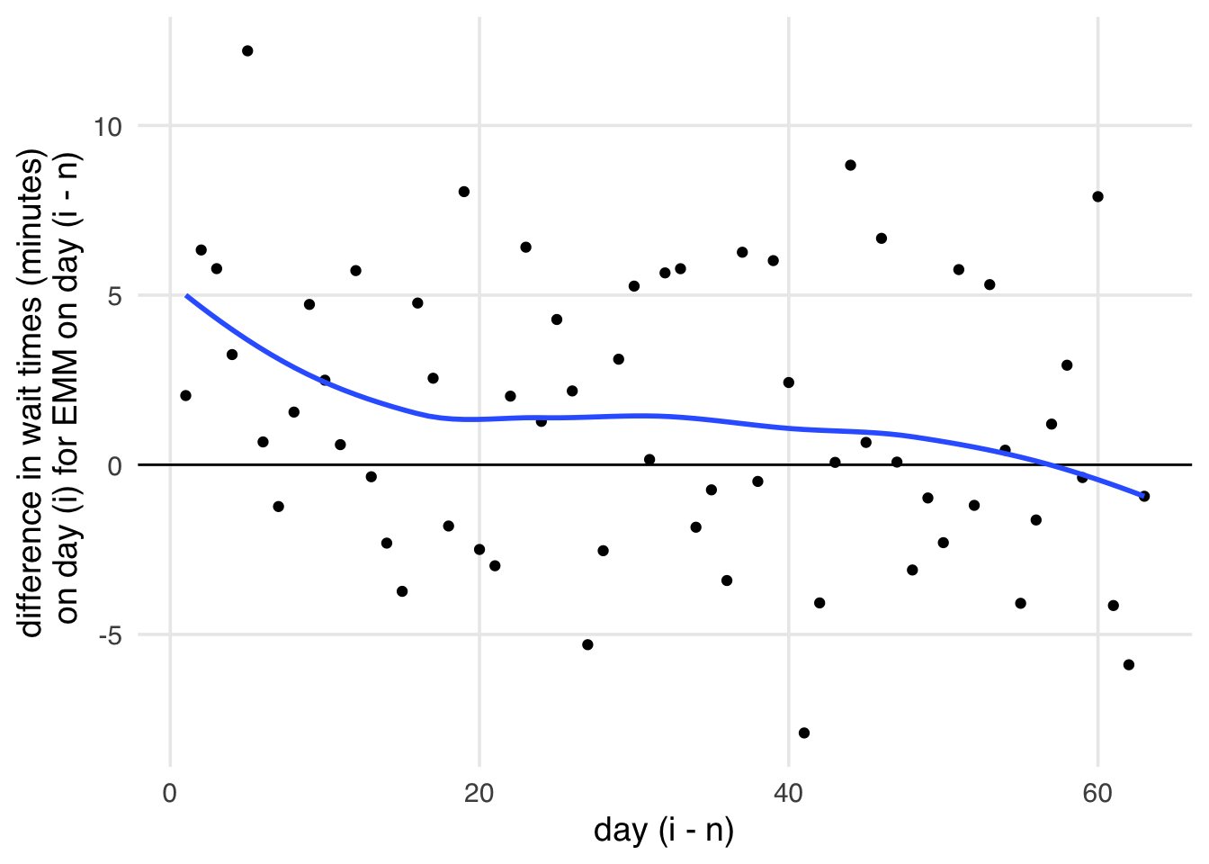
i and whether there were Extra Magic Hours on day i - n, where n represents the number of days previous to day i. We expect this relationship to rapidly approach the null, but the effect hovers above null for quite some time. This lingering effect implies we have some residual confounding present.
Now, let’s examine an example of a negative control outcome: the wait time for a ride at Universal Studios. Universal Studios is also in Orlando, so the set of causes for wait times are likely comparable to those at Disney World on the same day. Of course, whether or not there are Extra Magic Mornings at Disney shouldn’t affect the wait times at Universal on the same day: they are separate parks, and most people don’t visit both within an hour of one another. This negative control is an example of an effect implausible by the hypothesized mechanism.
We don’t have Universal’s ride data, so let’s simulate what would happen with and without residual confounding. We’ll generate wait times based on the historical temperature, park close time, and ticket season (the second two are technically specific to Disney, but we expect a strong correlation with the Universal versions). Because this is a negative outcome, it is not related to whether or not there were Extra Magic Morning hours at Disney.
seven_dwarfs_sim <- seven_dwarfs_train_2018 |>
  mutate(
    # we scale each variable and add a bit of random noise
    # to simulate reasonable Universal wait times
    wait_time_universal =
      park_temperature_high / 150 +
        as.numeric(park_close) / 1500 +
        as.integer(factor(park_ticket_season)) / 1000 +
        rnorm(n(), 5, 5)
  )
If we calculate the IPW effect of park_extra_magic_morning on wait_time_universal, we get 0.03 minutes, a roughly null effect, as expected. But what if we missed an unmeasured confounder, u, which caused Extra Magic Mornings and wait times at both Disney and Universal? Let’s simulate that scenario but augment the data further.
seven_dwarfs_sim2 <- seven_dwarfs_train_2018 |>
  mutate(
    u = rnorm(n(), mean = 10, sd = 3),
    wait_minutes_posted_avg = wait_minutes_posted_avg + u,
    park_extra_magic_morning = if_else(
      u > 10,
      rbinom(1, 1, .1),
      park_extra_magic_morning
    ),
    wait_time_universal =
      park_temperature_high / 150 +
        as.numeric(park_close) / 1500 +
        as.integer(factor(park_ticket_season)) / 1000 +
        u +
        rnorm(n(), 5, 5)
  )
Now, the effect for both Disney and Universal wait times is different. If we had seen -0.92 minutes for the effect for Disney, we wouldn’t necessarily know that we had a confounded result. However, since we know the wait times at Universal should be unrelated, it’s suspicious that the result, -2.64 minutes, is not null. That is evidence that we have unmeasured confounding.
Negative controls use the logical implications of the causal structure you assume. We can extend that idea to the entire DAG. If the DAG is correct, there are many implications for statistically determining how different variables in the DAG should and should not be related to each other. Like negative controls, we can check if variables that should be independent are independent in the data. Sometimes, the way that DAGs imply independence between variables is conditional on other variables. Thus, this technique is sometimes called implied conditional independencies (Textor et al. 2017). Let’s query our original DAG to find out what it says about the relationships among the variables.
query_conditional_independence(emm_wait_dag) |>
  unnest(conditioned_on)
# A tibble: 3 × 4
set a b conditioned_on
<chr> <chr> <chr> <chr>
1 1 park_close park_temp… <NA>
2 2 park_close park_tick… <NA>
3 3 park_temperature_high park_tick… <NA> In this DAG, three relationships should be null: 1) park_close and park_temperature_high, 2) park_close and park_ticket_season, and 3) park_temperature_high and park_ticket_season. None of these relationships need to condition on another variable to achieve independence; in other words, they should be unconditionally independent. We can use simple techniques like correlation and regression, as well as other statistical tests, to see if nullness holds for these relationships. Conditional independencies quickly grow in number in complex DAGs, and so dagitty implements a way to automate checks for DAG-data consistency given these implied nulls. dagitty checks if the residuals of a given conditional relationship are correlated, which can be modeled automatically in several ways. We’ll tell dagitty to calculate the residuals using non-linear models with type = "cis.loess". Since we’re working with correlations, the results should be around 0 if our DAG is right. As we see in Figure 16.5, though, one relationship doesn’t hold. There is a correlation between the park’s close time and ticket season.
test_conditional_independence(
  emm_wait_dag,
  data = seven_dwarfs_train_2018 |>
    filter(wait_hour == 9) |>
    mutate(
      across(where(is.character), factor),
      park_close = as.numeric(park_close),
    ) |>
    as.data.frame(),
  type = "cis.loess",
  # use 200 bootstrapped samples to calculate CIs
  R = 200
) |>
  ggdag_conditional_independence()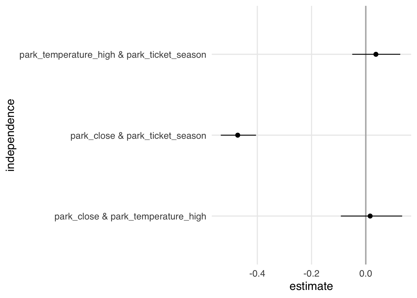
Why might we be seeing a relationship when there isn’t supposed to be one? A simple explanation is chance: just like in any statistical inference, we need to be cautious about over-extrapolating what we see in our limited sample. Since we have data for every day in 2018, we could probably rule that out. Another reason is that we’re missing direct arrows from one variable to the other, e.g. from historic temperature to park close time. Adding additional arrows is reasonable: park close time and ticket season closely track the weather. That’s a little bit of evidence that we’re missing an arrow.
At this point, we need to be cautious about overfitting the DAG to the data. DAG-data consistency tests cannot prove your DAG right and wrong, and as we saw in Chapter 5, statistical techniques alone cannot determine the causal structure of a problem. So why use these tests? As with negative controls, they provide a way to probe your assumptions. While we can never be sure about them, we do have information in the data. Finding that conditional independence holds is a little more evidence supporting your assumptions. There’s a fine line here, so we recommend being transparent about these types of checks: if you make changes based on the results of these tests, you should report your original DAG, too. Notably, in this case, adding direct arrows to all three of these relationships results in an identical adjustment set.
Let’s look at an example that is more likely to be misspecified, where we remove the arrows from park close time and ticket season to Extra Magic Morning.
emm_wait_dag2 <- dagify(
  wait_minutes_posted_avg ~ park_extra_magic_morning + park_close +
    park_ticket_season + park_temperature_high,
  park_extra_magic_morning ~ park_temperature_high,
  coords = coord_dag,
  labels = labels,
  exposure = "park_extra_magic_morning",
  outcome = "wait_minutes_posted_avg"
)

query_conditional_independence(emm_wait_dag2) |>
  unnest(conditioned_on)
# A tibble: 5 × 4
set a b conditioned_on
<chr> <chr> <chr> <chr>
1 1 park_close park_e… <NA>
2 2 park_close park_t… <NA>
3 3 park_close park_t… <NA>
4 4 park_extra_magic_morning park_t… <NA>
5 5 park_temperature_high park_t… <NA> This alternative DAG introduces two new relationships that should be independent. In Figure 16.6, we see an additional association between ticket season and Extra Magic Morning.
test_conditional_independence(
  emm_wait_dag2,
  data = seven_dwarfs_train_2018 |>
    filter(wait_hour == 9) |>
    mutate(
      across(where(is.character), factor),
      park_close = as.numeric(park_close),
    ) |>
    as.data.frame(),
  type = "cis.loess",
  R = 200
) |>
  ggdag_conditional_independence()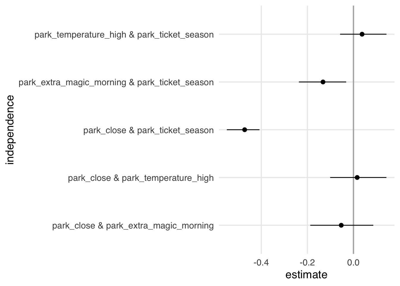
So, is this DAG wrong? Based on our understanding of the problem, it seems likely that’s the case, but interpreting DAG-data consistency tests has a hiccup: different DAGs can have the same set of conditional independencies. In the case of our DAG, one other DAG can generate the same implied conditional independencies (Figure 16.7). These are called equivalent DAGs because their implications are the same.
ggdag_equivalent_dags(emm_wait_dag2)curvatures <- rep(0, 10)
curvatures[c(4, 9)] <- .25
ggdag_equivalent_dags(emm_wait_dag2, use_edges = FALSE, use_text = FALSE) +
geom_dag_edges_arc(data = function(x) distinct(x), curvature = curvatures, edge_color = "grey80") +
geom_dag_edges_link(data = function(x) filter(x, (name == "park_extra_magic_morning" & to == "park_temperature_high") | (name == "park_temperature_high" & to == "park_extra_magic_morning")), edge_color = "black") +
geom_dag_text_repel(aes(label = label), data = function(x) filter(x, label %in% c("Extra Magic\nMorning", "Historic high\ntemperature")), box.padding = 15, seed = 12, color = "#494949") +
theme_dag()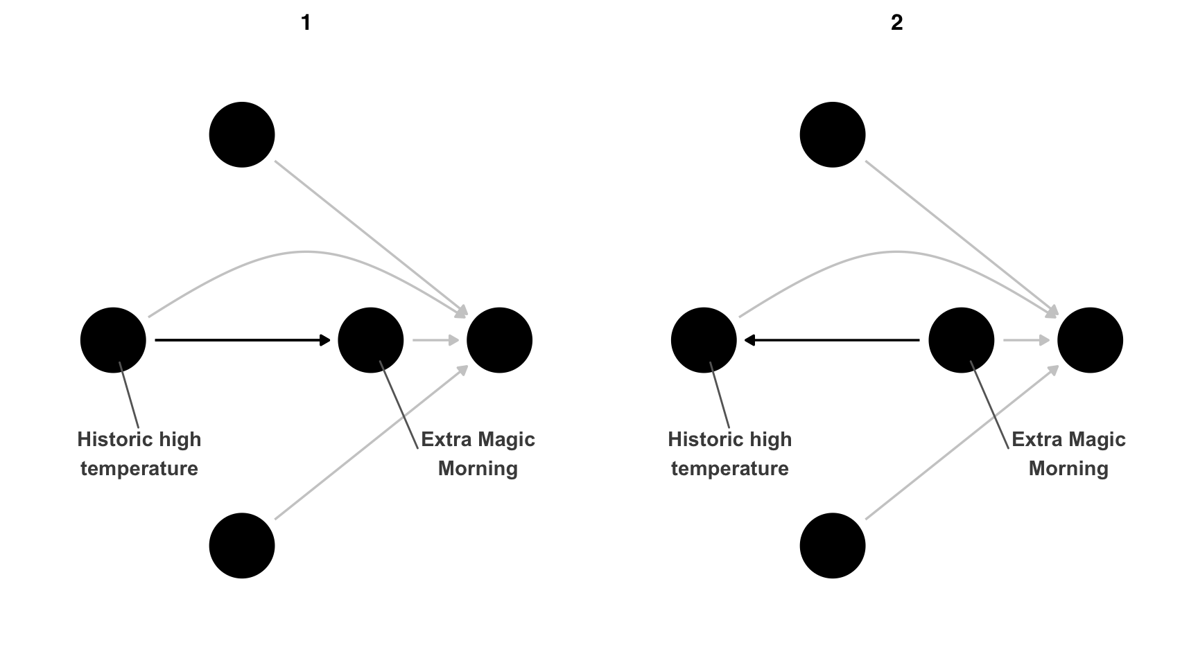
Equivalent DAGs are generated by reversing arrows. The subset of DAGs with reversible arrows that generate the same implications is called an equivalence class. While technical, this connection can condense the visualization to a single DAG where the reversible edges are denoted by a straight line without arrows.
ggdag_equivalent_class(emm_wait_dag2, use_text = FALSE, use_labels = TRUE)curvatures <- rep(0, 4)
curvatures[3] <- .25
emm_wait_dag2 |>
node_equivalent_class() |>
ggdag(use_edges = FALSE, use_text = FALSE) +
geom_dag_edges_arc(data = function(x) filter(x, !reversable), curvature = curvatures, edge_color = "grey90") +
geom_dag_edges_link(data = function(x) filter(x, reversable), arrow = NULL) +
geom_dag_text_repel(aes(label = label), data = function(x) filter(x, label %in% c("Extra Magic\nMorning", "Historic high\ntemperature")), box.padding = 16, seed = 12, size = 5, color = "#494949") +
theme_dag()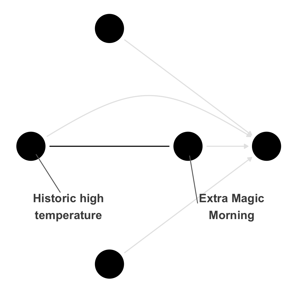
So, what do we do with this information? Since many DAGs can produce the same set of conditional independencies, one strategy is to find all the adjustment sets that would be valid for every equivalent DAG. dagitty makes this straightforward by calling equivalenceClass() and adjustmentSets(), but in this case, there are no overlapping adjustment sets.
library(dagitty)
# determine valid sets for all equiv. DAGs
equivalenceClass(emm_wait_dag2) |>
  adjustmentSets(type = "all")
We can see that by looking at the individual equivalent DAGs.
dags <- equivalentDAGs(emm_wait_dag2)

# no overlapping sets
dags[[1]] |> adjustmentSets(type = "all")
{ park_temperature_high }
{ park_close, park_temperature_high }
{ park_temperature_high, park_ticket_season }
{ park_close, park_temperature_high,
park_ticket_season }dags[[2]] |> adjustmentSets(type = "all") {}
{ park_close }
{ park_ticket_season }
{ park_close, park_ticket_season }The good news is that, in this case, one of the equivalent DAGs doesn’t make logical sense: the reversible edge is from historical weather to Extra Magic Morning, but that is impossible for both time-ordering reasons (historical temperature occurs in the past) and for logical ones (Disney may be powerful, but to our knowledge, they can’t yet control the weather). Even though we’re using more data in these types of checks, we need to consider the logical and time-ordered plausibility of possible scenarios.
As we mentioned in Section 4.4.1, you should specify your DAG ahead of time with ample feedback from other experts. Let’s now take the opposite approach to the last example: what if we used the original DAG but received feedback after the analysis that we should add more variables? Consider the expanded DAG in Figure 16.9. We’ve added two new confounders: whether it’s a weekend or a holiday. This analysis differs from when we checked alternate adjustment sets in the same DAG; in that case, we checked the DAG’s logical consistency. In this case, we’re considering a different causal structure.
labels <- c(
  park_extra_magic_morning = "Extra Magic\nMorning",
  wait_minutes_posted_avg = "Average\nwait",
  park_ticket_season = "Ticket\nSeason",
  park_temperature_high = "Historic high\ntemperature",
  park_close = "Time park\nclosed",
  is_weekend = "Weekend",
  is_holiday = "Holiday"
)

emm_wait_dag3 <- dagify(
  wait_minutes_posted_avg ~ park_extra_magic_morning + park_close + park_ticket_season + park_temperature_high + is_weekend + is_holiday,
  park_extra_magic_morning ~ park_temperature_high + park_close + park_ticket_season + is_weekend + is_holiday,
  park_close ~ is_weekend + is_holiday,
  coords = time_ordered_coords(),
  labels = labels,
  exposure = "park_extra_magic_morning",
  outcome = "wait_minutes_posted_avg"
)

curvatures <- rep(0, 13)
curvatures[11] <- .25

emm_wait_dag3 |>
  tidy_dagitty() |>
  node_status() |>
  ggplot(
    aes(x, y, xend = xend, yend = yend, color = status)
  ) +
  geom_dag_edges_arc(curvature = curvatures, edge_color = "grey80") +
  geom_dag_point() +
  geom_dag_text_repel(aes(label = label), size = 3.8, seed = 16301, color = "#494949") +
  scale_color_okabe_ito(na.value = "grey90") +
  theme_dag() +
  theme(legend.position = "none") +
  coord_cartesian(clip = "off")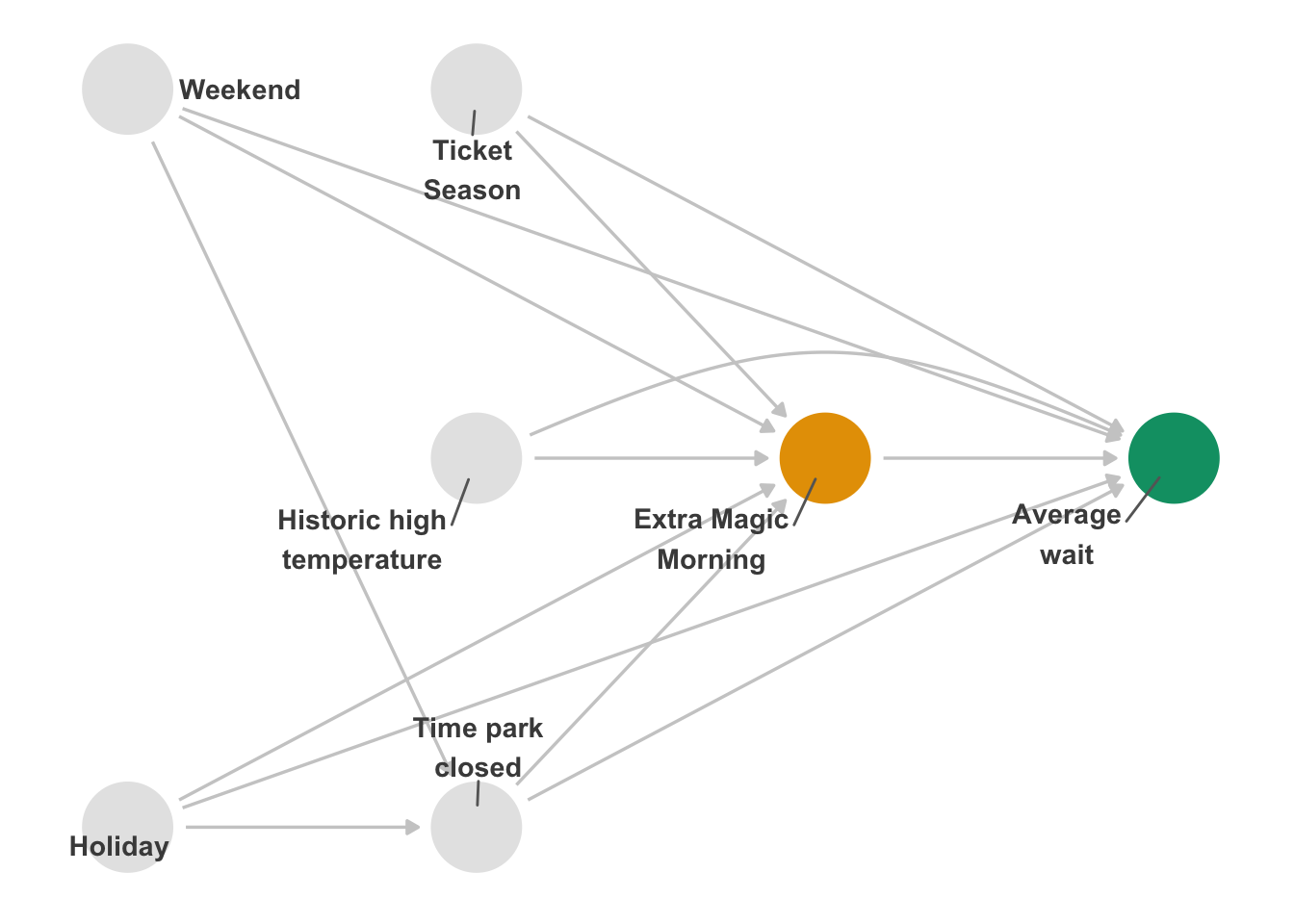
We can calculate these features from park_date using the timeDate package.
library(timeDate)

holidays <- c(
  "USChristmasDay",
  "USColumbusDay",
  "USIndependenceDay",
  "USLaborDay",
  "USLincolnsBirthday",
  "USMemorialDay",
  "USMLKingsBirthday",
  "USNewYearsDay",
  "USPresidentsDay",
  "USThanksgivingDay",
  "USVeteransDay",
  "USWashingtonsBirthday"
) |>
  holiday(2018, Holiday = _) |>
  as.Date()

seven_dwarfs_with_days <- seven_dwarfs_train_2018 |>
  mutate(
    is_holiday = park_date %in% holidays,
    is_weekend = isWeekend(park_date)
  ) |>
  filter(wait_hour == 9)
Both Extra Magic Morning hours and posted wait times are associated with whether it’s a holiday or weekend.
tbl_data_days <- seven_dwarfs_with_days |>
  select(wait_minutes_posted_avg, park_extra_magic_morning, is_weekend, is_holiday)

library(labelled)
var_label(tbl_data_days) <- list(
  is_weekend = "Weekend",
  is_holiday = "Holiday",
  park_extra_magic_morning = "Extra Magic Morning",
  wait_minutes_posted_avg = "Posted Wait Time"
)

tbl1 <- gtsummary::tbl_summary(
  tbl_data_days,
  by = is_weekend,
  include = -is_holiday
)

tbl2 <- gtsummary::tbl_summary(
  tbl_data_days,
  by = is_holiday,
  include = -is_weekend
)

gtsummary::tbl_merge(list(tbl1, tbl2), c("Weekend", "Holiday"))| Characteristic |
Weekend
|
Holiday
|
||
|---|---|---|---|---|
|
TRUE N = 1011 |
FALSE N = 2531 |
TRUE N = 111 |
FALSE N = 3431 |
|
| Posted Wait Time | 65 (56, 75) | 67 (60, 77) | 76 (60, 77) | 66 (58, 77) |
| Extra Magic Morning | 5 (5.0%) | 55 (22%) | 1 (9.1%) | 59 (17%) |
| 1 Median (Q1, Q3); n (%) | ||||
When we refit the IPW estimator, we get 7.58 minutes, slightly bigger than we got without the two new confounders. Because it was a deviation from the analysis plan, you should likely report both effects. That said, this new DAG is probably more correct than the original one. From a decision point of view, though, the difference is slight in absolute terms (about a minute) and the effect in the same direction as the original estimate. In other words, the result is not terribly sensitive to this change regarding how we might act on the information.
One other point here: sometimes, people present the results of using increasingly complicated adjustment sets. This comes from the tradition of comparing complex models to parsimonious ones. That type of comparison is a sensitivity analysis in its own right, but it should be principled: rather than fitting simple models for simplicity’s sake, you should compare competing adjustment sets or conditions. For instance, you may feel like these two DAGs are equally plausible or want to examine if adding other variables better captures the baseline crowd flow at the Magic Kingdom.
Thus far, we’ve probed some of the assumptions we’ve made about the causal structure of the question. We can take this further using quantitative bias analysis, which uses mathematical assumptions to see how results would change under different conditions.
Sensitivity analyses for unmeasured confounding are important tools in observational studies to assess how robust findings are to potential unmeasured factors (D’Agostino McGowan 2022). These analyses rely on three key components:
By specifying plausible values for these relationships, researchers can quantify how much the observed effect might change if such an unmeasured confounder existed.
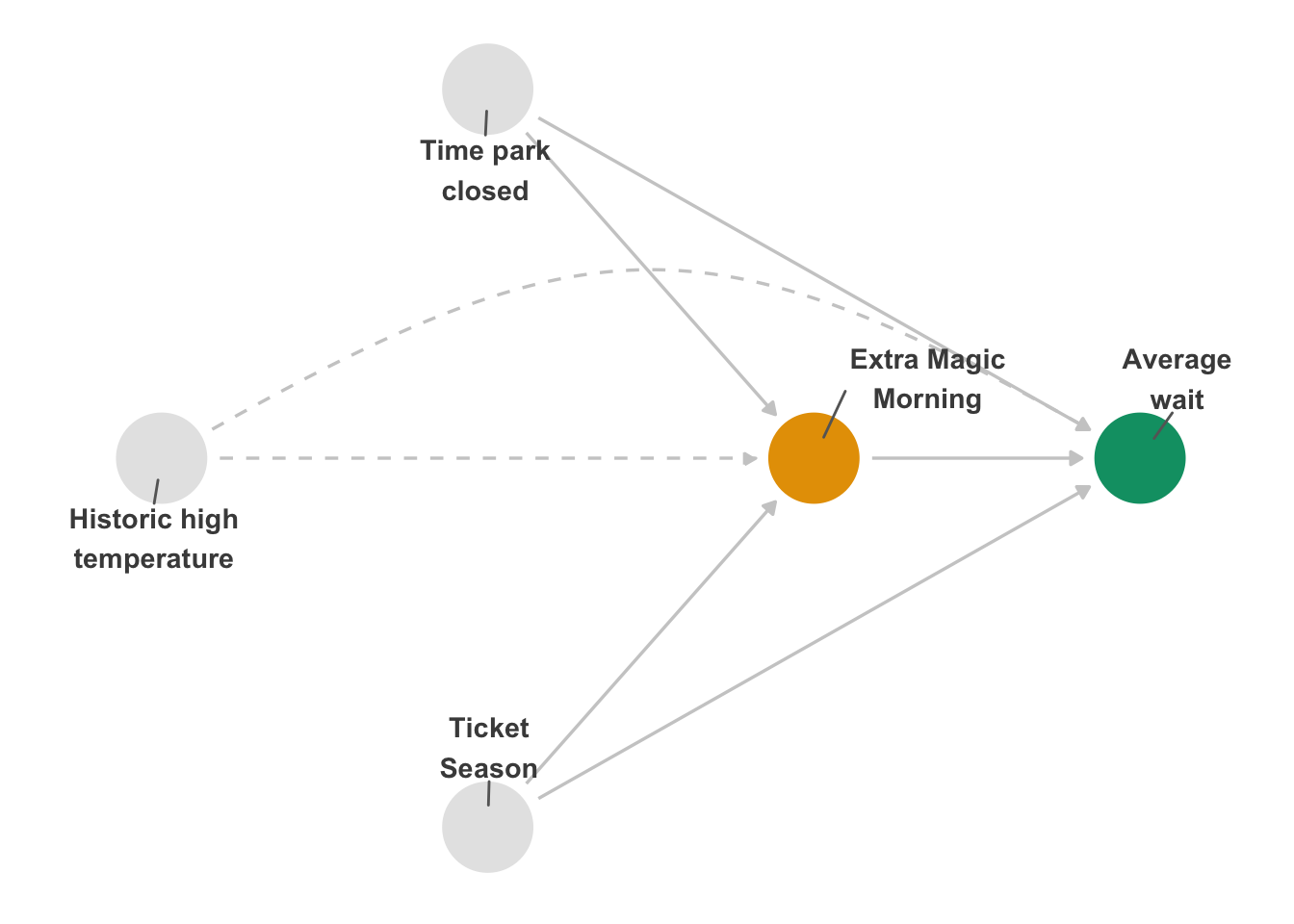
Let’s think about why this works in the context of our example above. Let’s assume Figure 16.10 displays the true relationship between our exposure and outcome of interest. Suppose we hadn’t measured historic high temperature, denoted by the dashed lines; we have an unmeasured confounder. The three key components above are described by 1) the arrow between ‘Extra Magic Morning’ and ‘Average wait’, 2) The arrow between ‘Historic high temperature’ and ‘Extra Magic Morning’, and 3) the arrow between ‘Historic high temperature’ and ‘Average wait’.
curvatures <- rep(0, 7)
curvatures[5] <- 0.3
emm_wait_dag |>
  tidy_dagitty() |>
  node_status() |>
  mutate(linetype = if_else(name == "park_temperature_high", "dashed", "solid")) |>
  ggplot(
    aes(x, y, xend = xend, yend = yend, color = status, edge_linetype = linetype)
  ) +
  geom_dag_edges_arc(curvature = curvatures, edge_color = "grey80") +
  geom_dag_point() +
  geom_dag_text_repel(aes(label = label), size = 3.8, seed = 1630, color = "#494949") +
  scale_color_okabe_ito(na.value = "grey90") +
  theme_dag() +
  theme(legend.position = "none") +
  coord_cartesian(clip = "off") +
  scale_x_continuous(
    limits = c(-1.25, 2.25),
    breaks = c(-1, 0, 1, 2)
  )
Various methods are available depending on the type of outcome (e.g. continuous, binary, time-to-event) and how much is known about potential unmeasured confounders. While these analyses cannot prove the absence of unmeasured confounding, they provide valuable insight into how sensitive results are to violations of the “no unmeasured confounders” assumption that is crucial for causal inference in observational studies.
The first componenet, the observed exposure-outcome effect, is the proposed causal effect of interest, i.e. the effect you would like to perform a sensitivity analysis on. The effect itself will depend on the choice of outcome model, which in turn often depends on the distribution of the outcome and the desired effect measure:
For continuous outcomes: Linear models or generalized linear models (GLMs) with Gaussian distribution and identity link are used, typically estimating a coefficient.
For binary outcomes, we have a few choices:
Let’s use the analysis from Table 16.1 where we only adjusted for ‘Time park closed’ and ‘Ticket season’. According to Figure 16.10, we know ‘Historic high temperature’ is also a confounder, but it is unmeasured so we cannot include it in our practical adjustment set. This resulted in an observed effect of 6.58.
The relationship between an unmeasured confounder and the exposure can be characterized in three ways:
These characterizations allow researchers to specify the unmeasured confounder-exposure relationship in sensitivity analyses, accommodating different types of confounders and levels of knowledge about their distribution.
Our unmeasured confounder here, ‘Historic high temperature’, is continuous. For this example, let’s assume it is normally distributed. We say to assume “unit variance” (a variance of 1), because it makes it easier to talk about the impact of the confounder in standard-deviation terms. Let’s assume that on days with extra magic morning hours the historic high temperature is normally distributed with a mean of 80.5 degrees and a standard deviation of 9 degrees. Likewise, assume that on days without extra magic morning hours the historic high temperature is normally distributed with a mean of 82 degrees and a standard deviation of 9 degrees. We can convert these to ‘unit variance’ normally distributed variables by dividing by that standard deviation, 9 (sometimes we refer to this as standardizing our variable); this gives us a standardized mean of 8.94 for days with extra magic morning hours and 9.11 for the others, or a mean difference of -0.17. Hold on to this number; we’ll use it in conjunction with the next section for our sensitivity analysis.
The relationship between an unmeasured confounder and the outcome can be quantified in two main ways:
Coefficient-based approach: Estimate the coefficient for an unmeasured confounder in a fully adjusted outcome model. You can also estimate the exponentiated coefficient (risk ratio, odds ratio, or hazard ratio)
Distribution-agnostic approach (for continuous outcomes): Use partial
Let’s do the coeffient-based approach. In our case, we need to estimate what we think the coefficient bewteen our standardized ‘Historic high temperature’ variable and our outcome after adjusting for our exposure as well as the other measured confounders (in this case ticket season and the time the park closed). Another way to describe this effect in the context of this problem is: “How would the average posted wait time change if we changed the historic high temperature by one standard deviation, after adjusting for whether there were extra magic morning hours, the park close time, and the ticket season?” Let’s suppose we think this would change by -2.3 minutes. That is, if the historic high temperature is one standard deviation unit higher (in our scenario, 9 degrees warmer), we expect this to decrease the average posted wait time by 2.3 minutes.
For a mathematical explanation of these quantities, see D’Agostino McGowan (2022).
Once you have estimated the above three quantities, we can calculate a updated effect estimate between the exposure and outcome that takes into account an unmeasured factor like the one specified. We can use the {tipr} R package to perform these analyses. The functions in the {tipr} package follow a unified grammar. The function names follow this form: {action}_{effect}_with_{what}.
For example, to adjust (action) a coefficient (effect) with a binary unmeasured confounder (what), we use the function adjust_coef_with_binary().
Below is a copy of the table included in Lucy and McGowan (2022) about this package.
| category | Function term | Use |
|---|---|---|
| action | adjust |
These functions adjust observed effects, requiring both the unmeasured | confounder-exposure relationship and unmeasured confounder-outcome relationship to be specified. |
tip |
These functions tip observed effects. Only one relationship, either the unmeasured confounder-exposure relationship or unmeasured confounder-outcome relationship needs to be specified. | |
| effect | coef |
These functions specify an observed coefficient from a linear, log-linear, logistic, or Cox proportional hazards model |
rr |
These functions specify an observed relative risk | |
or |
These functions specify an observed odds ratio | |
hr |
These functions specify an observed hazard ratio | |
| what | continuous |
These functions specify an unmeasured standardized Normally distributed confounder. These functions will include the parameters exposure_confounder_effect and confounder_outcome_effect
|
binary |
These functions specify an unmeasured binary confounder. These functions will include the parameters exposed_confounder_prev, unexposed_confounder_prev, and confounder_outcome_effect
|
|
r2 |
These functions specify an unmeasured confounder parameterized by specifying the percent of variation in the exposure / outcom explained by the unmeasured confounder. These functions will include the parameters confounder_exposure_r2 and outcome_exposure_r2
|
tipr functions.
You can find full documentation here: r-causal.github.io/tipr/
Ok, now we have everything we need to perform our sensitivity analysis. Table 16.3 provides what we need; we can use the {tipr} R package to apply these; we will use the adjust_coef function. Let’s plug in the quantities we established above for each of the three parameters, effect_observed, exposure_confounder_effect, and confounder_outcome_effect.
library(tipr)
adjust_coef(
  effect_observed = 6.58,
  exposure_confounder_effect = -.17,
  confounder_outcome_effect = -2.3
)
# A tibble: 1 × 4
effect_adjusted effect_observed
<dbl> <dbl>
1 6.19 6.58
# ℹ 2 more variables:
# exposure_confounder_effect <dbl>,
# confounder_outcome_effect <dbl>Examining this output, we see that if there were an unmeasured confounder like the one we specified above, our observed effect, 6.58, would be attenuated to 6.19. That is, rather than the effect of extra magic morning hours increasing the average posted wait time at 9am by 6.58 minutes, the true effect would be 6.19 minutes, assuming our specifications about the unmeasured confounder were correct. Take a look at Table 16.1, this number should look familiar.
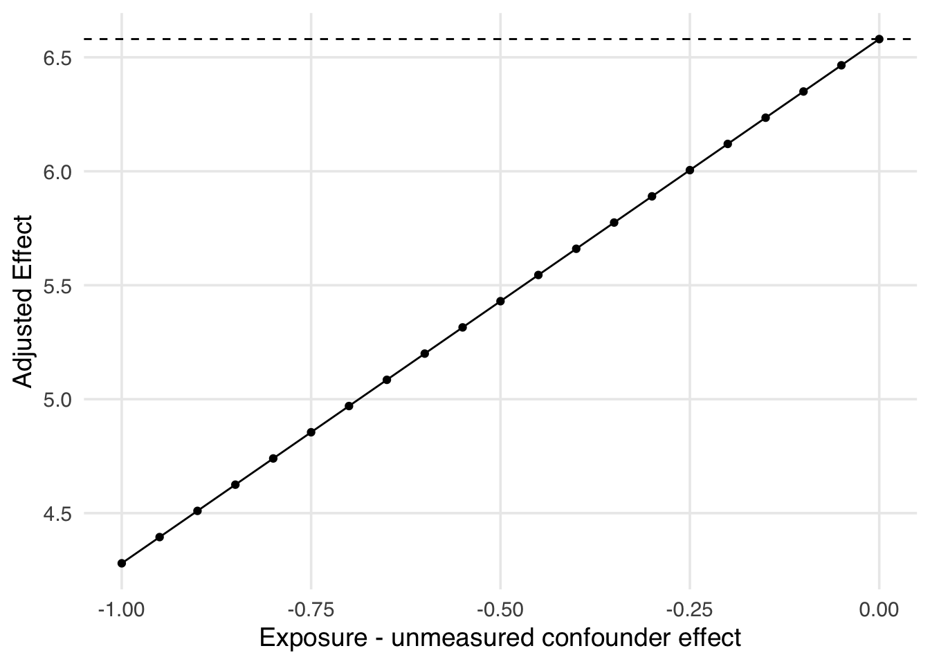
In this case, our “guesses” about the relationship between our unmeasured confounder and the exposure and outcome were accurate because it was, in fact, measured! In reality, we often have to use other techniques to come up with these guesses. Sometimes, we have access to different data or previous studies that would allow us to quantify these effects. Sometimes, we have some information about one of the effects, but not the other (i.e., we have a guess for the impact of the historic high temperature on the average posted wait time, but not on whether there are extra magic morning hours). In these cases, one solution is an array-based approach where we specify the effect we are sure of and vary the one we are not. Let’s see an example of that. We can plot this array to help us see the impact of this potential confounder. Examining Figure 16.11, we can see, for example, that if there was a one standard deviation difference in historic high temperature such that extra magic morning hours were 9 degrees cooler on average than days without extra magic morning hours, the true causal effect of extra magic morning hours on the average posted wait time at 9am would be 4.28 minutes, rather than the observed 6.58 minutes.
library(tipr)
adjust_df <- adjust_coef(
  effect_observed = 6.58,
  exposure_confounder_effect = seq(0, -1, by = -0.05),
  confounder_outcome_effect = -2.3,
  verbose = FALSE
)

ggplot(
  adjust_df,
  aes(
    x = exposure_confounder_effect,
    y = effect_adjusted
  )
) +
  geom_hline(yintercept = 6.58, lty = 2) +
  geom_point() +
  geom_line() +
  labs(
    x = "Exposure - unmeasured confounder effect",
    y = "Adjusted Effect"
  )
Many times, we find ourselves without any certainty about a potential unmeasured confounder’s impact on the exposure and outcome. One approach could be to decide on a range of both values to examine. Figure 16.12 is an example of this. One thing we can learn by looking at this graph is that the adjusted effect will cross the null when a one standard deviation change in the historic high temperature changes the average posed wait time by at least ~7 minutes and there is around a one standard deviation difference between the average historic temperature on extra magic morning days compared to those without. This is known as a tipping point.
library(tipr)
adjust_df <- adjust_coef(
  effect_observed = 6.58,
  exposure_confounder_effect = rep(seq(0, -1, by = -0.05), each = 7),
  confounder_outcome_effect = rep(seq(-1, -7, by = -1), times = 21),
  verbose = FALSE
)

ggplot(
  adjust_df,
  aes(
    x = exposure_confounder_effect,
    y = effect_adjusted,
    group = confounder_outcome_effect
  )
) +
  geom_hline(yintercept = 6.58, lty = 2) +
  geom_hline(yintercept = 0, lty = 3) +
  geom_point() +
  geom_line() +
  geom_label(
    data = adjust_df[141:147, ],
    aes(
      x = exposure_confounder_effect,
      y = effect_adjusted,
      label = confounder_outcome_effect
    )
  ) +
  labs(
    x = "Exposure - unmeasured confounder effect",
    y = "Adjusted Effect"
  )
Tipping point sensitivity analyses aim to determine the characteristics of an unmeasured confounder that would change the observed effect to a specific value, often the null. Instead of exploring a range of values for unknown sensitivity parameters, it identifies the value that would “tip” the observed effect. This approach can be applied to point estimates or confidence interval bounds. The analysis calculates the smallest possible effect of an unmeasured confounder that would cause this tipping. By rearranging equations and setting the adjusted outcome to the null (or any value of interest), we can solve for a single sensitivity parameter, given other parameters. The {tipr} R package also provides functions to perform these calculations for various scenarios, including different effect measures, confounder types, and known relationships.
Using the example above, let’s use the tip_coef function to see what would tip our observed coefficient. For this, we only need to specify one, either the exposure-unmeasured confounder effect or the unmeasured confounder-outcome effect and the function will calculate the other that would result in “tipping” the observed effect to the null. Let’s first replicate what we saw in Figure 16.12. Let’s specify the unmeasured confounder effect-outcome effect of -7 minutes. The output below tells us that if there is an unmeasured confounder with an effect on the outcome of -7 minutes, it would need to have a diffence of -0.94 in order to tip our observed effect of 6.58 minutes.
tip_coef(
  effect_observed = 6.58,
  confounder_outcome_effect = -7
)
# A tibble: 1 × 4
effect_observed exposure_confounder_effect
<dbl> <dbl>
1 6.58 -0.94
# ℹ 2 more variables: confounder_outcome_effect <dbl>,
# n_unmeasured_confounders <dbl>Instead, let’s suppose we were pretty sure about the unmeasured confounder-outcome effect we assumed above, -2.3, but we weren’t sure what to expect in terms of the relationship between historic high temperature and whether the day had extra magic morning hours. Let’s see how big the difference there would have to be for a confounder like this to make our observed effect of 6.58 minutes tip to 0 minutes.
tip_coef(
  effect_observed = 6.58,
  confounder_outcome_effect = -2.3
)
# A tibble: 1 × 4
effect_observed exposure_confounder_effect
<dbl> <dbl>
1 6.58 -2.86
# ℹ 2 more variables: confounder_outcome_effect <dbl>,
# n_unmeasured_confounders <dbl>This shows that we would need an effect of -2.86 between the expsoure and the confounder. In other words, for this particular example, we would need the average difference in historic temperature to be ~25 degrees (-2.86 times our standard deviation, 9), to change our effect to the null. This is a pretty huge, and potentially implausible, effect. If we were missing historic high temperature, and assuming we are correct about our -2.3 estimate, we could feel pretty confident that missing this variable is not skewing our result so much that we are directionally wrong.
